Regression
Introduction
Regression analysis is a conceptually simple method for investigating functional relationships between variables. The relationship is expressed in the form of an equation or a model connecting the response or dependent variable and one or more explanatory or predictor variables.
We denote the response variable by \(Y\), and the set of predictor variables by \(X_1, X_2, \dots, X_p\), where \(p\) denotes the number of predictor variables.
The general regression model is specified as:
\begin{equation} \label{dfn:general_regression} Y = f(X_1, X_2, \dots, X_p) + \epsilon \end{equation}
An example is the linear regression model:
\begin{equation} Y = \beta_0 + \beta_1X_1 + \dots + \beta_pX_p + \epsilon \end{equation}
where \(\beta_0, \dots, \beta_p\) called the regression paramaters or coefficients, are unknown constants to be estimated from the data. \(\epsilon\) is the random error representing the discrepancy in the approximation.
Steps in Regression Analysis
1. Statement of the problem
Formulation of the problem includes determining the questions to be addressed.
2. Selection of Potentially Relevant Variables
We select a set of variables that are thought by the experts in the area of study to explain or predict the response variable.
Each of these variables could be qualitative or quantitative. A technique used in casse where the response variable is binary is called logistic regression. If all predictor variables are qualitative, the techniques used in the analysis of the data are called the analysis of variance techniques. If some of the predictor variables are quantitative while others are qualitative, regression analysis in these cases is called the analysis of covariance.
| Type | Conditions |
|---|---|
| Univariate | Only 1 quantitative RV |
| Multivariate | 2 or more quantitative RV |
| Simple | Only 1 predictor variable |
| Multiple | 2 or more predictor variables |
| Linear | All parameters enter the equation linearly, possibly after transformation of the data |
| Non-linear | The relationship between the response and some of the predictors is non-linear (no transformation to make parameters appear linearly) |
| Analysis of variance | All predictors are qualitative variables |
| Analysis of covariance | Some predictors are quantitative variables, others are qualitative |
| Logistic | The RV is qualitative |
3. Model specification
The form of the model that is thought to relate the response variable to the set of predictor variables can be specified initially by experts in the area of study based on their knowledge or their objective and/or subjective judgments.
We need to select the form of the function \(f(X_1, X_2, \dots, X_p)\) in .
4. Method of Fitting
We want to perform parameter estimation or model fitting after defining the model and collecting the data. the most commonly used method of estimation is called the least squares method. Other estimation methods we consider are the maximum likelihood method, ridge regression and the principal components method.
5. Model Fitting
The estimates of the regression parameters \(\beta_0, \beta_1, \dots, \beta_p\) are denoted by \(\hat{\beta_0}, \hat{\beta_1}, \dots, \hat{\beta_p}\). the obtained \(\hat{Y}\) denotes the predicted value.
6. Model Criticism and Selection
The validity of statistical methods depend on certain assumptions, about the data and the model. We need to address the following questions:
- What are the required assumptions?
- For each of these assumptions, how do we determine if they are valid?
- What can be done in cases where assumptions do not hold?
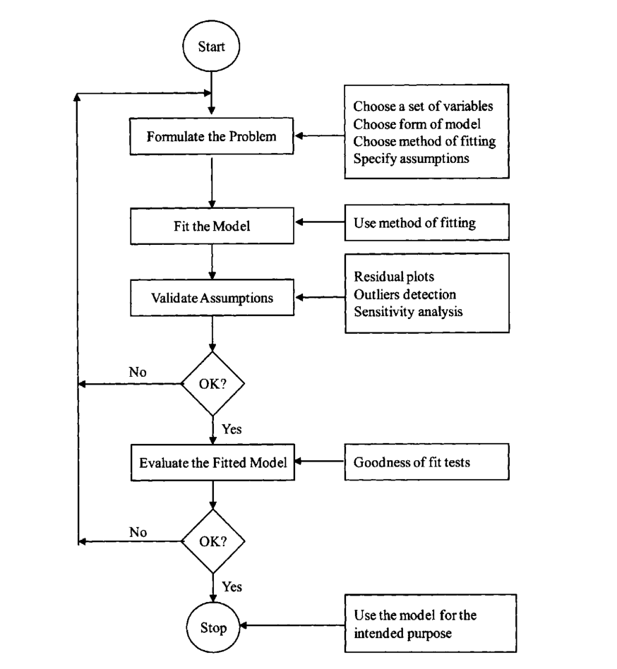
Figure 1: Flowchart illustrating the dynamic iterative regression process
Simple Linear Regression
Simple linear regression is a straightforward approach for predicting a quantitative response \(Y\) on the basis of a single predictor variable \(X\). Mathematically, we write this linear relationship as:
\begin{equation} \label{eqn:slr} Y \approx \beta_0 + \beta_1 X \end{equation}
We describe this as regressing \(Y\) on \(X\).
We wish to measure both the direction and strength of the relationship between \(Y\) and \(X\). Two related measures, known as the covariance and the correlation coefficient are developed later.
We use our training data to produce estimates \(\hat{\beta_0}\) and \(\hat{\beta_1}\) for the model coefficients, and we can predict outputs by computing:
\begin{equation} \hat{y} = \hat{\beta_0} + \hat{\beta_1} X \end{equation}
Let \(\hat{y_i} = \hat{\beta_0} + \hat{\beta_1}\) be the prediction of \(Y\) based on the ith value of \(X\). Then \(e_i = y_i - \hat{y_i}\) represents the ith residual. We can define the residual sum of squares (RSS) as:
\begin{equation} \label{eqn:dfn:rss} \mathrm{RSS} = e_1^2 + e_2^2 + \dots + e_n^2 \end{equation}
The least squares approach chooses \(\hat{\beta_0}\) and \(\hat{\beta_1}\) to minimise the RSS.
If \(f\) is to be approximated by a linear function, then we can write the relationship as:
\begin{equation} Y = \beta_0 + \beta_1 X + \epsilon \end{equation}
where \(\epsilon\) is an error term – the catch-all for what we miss with this simple model. For example, the true relationship is probably not linear, and other variables cause variation in \(Y\). It is typically assumed that the error term is independent of \(X\).
We need to assess the accuracy of our estimates. How far off will a single estimation of \(\hat{\mu}\) be? In general, we can answer this question by computing the standard error of \(\hat{\mu}\), written as \(\mathrm{SE}(\hat{\mu})\). This is given by:
\begin{equation} \label{eqn:dfn:se} \mathrm{Var}(\hat{\mu}) = \mathrm{SE}(\hat{\mu})^2 = \frac{\sigma^2}{n} \end{equation}
where \(\sigma\) is the standard deviation of each of the realizations \(y_i\) of \(Y\).
Standard errors can be used to compute confidence intervals. A 95% confidence interval is defined as a range of values such that with 95% probability, the range will contain the true unknown value of the parameter. For linear regression, the 95% confidence interval for \(\beta_1\) approximately takes the form:
\begin{equation} \hat{\beta_1} \pm 2 \cdot SE(\hat{\beta_1}) \end{equation}
Standard errors can also be used to perform hypothesis tests on the coefficients. The most common hypothesis test involves testing the null hypothesis of:
\begin{equation} \label{eqn:dfn:null_hyp} H_0 : \mathrm{There is no relationship between X and Y} (\beta_1 = 0) \end{equation}
versus the alternative hypothesis:
\begin{equation} \label{eqn:dfn:alt_hyp} H_a : \mathrm{There is a relationship between X and Y} (\beta_1 \ne 0) \end{equation}
To test the null hypothesis, we need to determine whether \(\hat{\beta_1}\) is sufficiently far from zero that we can be confident that \(\beta_1\) is non-zero. How far is far enough? This depends on the accuracy of \(\hat{\beta_1}\), or \(\mathrm{SE}(\hat{\beta_1})\). In practice, we compute a t-statistic, given by:
\begin{equation} \label{eqn:dfn:t-statistic} t = \frac{\hat{\beta_1} - 0}{\mathrm{SE}(\hat{\beta_1})} \end{equation}
which measures the number of standard deviations that \(\hat{\beta_1}\) is away from 0. If there really is no relationship between \(X\) and \(Y\), then we expect that Eq. will have a t-distribution with \(n-2\) degrees of freedom. The t-distribution has a bell shape and for values of \(n\) greater than approximately 30 it is similar to the normal distribution.
It is a simple matter to compute the probability of observing any number equal to \(\lVert t \rVert\) or larger in absolute value, assuming \(\beta_1 = 0\). We call this probability the p-value. A small p-value indicates that it is unlikely to observe such a substantial association between the predictor and the response due to chance.
Assessing the accuracy of the model
Once we have rejected the null hypothesis in favour of the alternative hypothesis, it is natural to want to quantify the extent to which the model fits the data.
Residual Standard Error (RSE)
After we compute the least square estimates of the parameters of a linear model, we can compute the following quantities:
\begin{align}
\mathrm{SST} &= \sum(y_i - \bar{y})^2 \\\
\mathrm{SSR} &= \sum(\hat{y_i} - \bar{y})^2 \\\
\mathrm{SSE} &= \sum(y_i - \hat{y_i})^2
\end{align}
A fundamental equality in both simple and multiple regressions is given by \(\mathrm{SST} = \mathrm{SSR} + \mathrm{SSE}\). This can be interpreted as: The deviation from the mean is equal to the deviation due to fit, plus the residual.
\(R^2\) statistic
The RSE provides an absolute measure of lack of fit of the model to the data. But since it is measured in the units of \(Y\), it is not always clear what constitutes a good RSE. The \(R^2\) statistic provides an alternative measure of fit. It takes a form of a proportion, and takes values between 0 and 1, independent of the scale of \(Y\).
\begin{equation} \label{eqn:dfn:r_squared} R^2 = \frac{\mathrm{SSR}}{\mathrm{SST}} = 1 - \frac{\mathrm{SSE}}{\mathrm{SST}} \end{equation}
where \(\mathrm{SST} = \sum(y_i - \bar{y})^2\) is the total sum of squares. SST measures the total variance in the response \(Y\), and can be thought of as the amount of variability inherent in the response before the regression is performed. Hence, \(R^2\) measures the proportion of variability in \(Y\) that can be explained using \(X\).
Note that the correlation coefficient \(r = \mathrm{Cor}(X, Y)\) is related to the \(R^2\) in the simple linear regression setting: \(r^2 = R^2\).
Multiple Linear Regression
We can extend the simple linear regression model to accommodate multiple predictors:
\begin{equation} Y = \beta_0 + \beta_1 X_1 + \beta_2 X_2 + \dots + \beta_p X_p + \epsilon \end{equation}
We choose \(\beta_0, \beta_1, \dots, \beta_p\) to minimise the sum of squared residuals:
\begin{equation} \mathrm{RSS} = \sum_{i=1}^{n} (y_i - \hat{y_i})^2 \end{equation}
Unlike the simple regression estimates, the multiple regression coefficient estimates have complicated forms that are most easily represented using matrix algebra.
Interpreting Regression Coefficients
\(\beta_0\), the constant coefficient, is the value of \(Y\) when \(X_1 = X_2 \dots = X_p = 0\), as in simple regression. The regression coefficient \(\beta_j\) has several interpretations.
First, it may be interpreted as the change in \(Y\) corresponding to a unit change in \(X_j\) when all other predictor variables are held constant. In practice, predictor variables may be inherently related, and it is impossible to hold some of them constant while varying others. The regression coefficient \(\beta_j\) is also called the partial regression coefficient, because \(\beta_j\) represents the contribution of \(X_j\) to the response variable \(Y\) adjusted for other predictor variables.
Centering and Scaling
The magnitudes of the regression coefficients in a regression equation depend on the unit of measurements of the variables. To make the regression coefficients unit-less, one may first center or scale the variables before performing regression computations.
When dealing with constant term models, it is convenient to center and scale the variables, but when dealing with no-intercept models, we need only to scale the variables.
A centered variable is obtained by subtracting from each observation the mean of all observations. For example, the centered response variable is \((Y - \bar{y})\), and the centered jth predictor variable is \((X_j - \bar{x}_j)\). The mean of a centered variable is 0.
The centered variables can also be scaled. Two types of scaling are usually performed: unit-length scaling and standardizing.
Unit-length scaling of response variable \(Y\) and the jth predictor variable \(X_j\) is obtained as follows:
\begin{align}
\tilde{Z}_y &= (Y - \bar{y})/L_y \\\
\tilde{Z}_j &= (X - \bar{x}_j)/L_j \\\
\end{align}
where:
\begin{equation} L_y = \sqrt{\sum_{i=1}^{n}(y_i - \bar{y})^2} \text{ and } L_j = \sqrt{\sum_{i=1}^{n}(x_{ij} - \bar{x}_j)^2}\text{ , } j = 1,2,\dots,p \end{equation}
The quantities \(L_y\) is referred to as the length of the centered variable \(Y_\bar{y}\) because it measures the size or the magnitudes of the observations in \(Y - \bar{y}\). \(L_j\) has a similar interpretation.
Unit length scaling has the following property:
\begin{equation} \mathrm{Cor}(X_j, X_k) = \sum_{i=1}^{n}z_{ij}z_{ik} \end{equation}
The second type of scaling is called standardizing, which is defined by:
\begin{align}
\tilde{Y} &= \frac{Y - \bar{y}}{s_y} \\\
\tilde{X}_j &= \frac{X_j - \bar{x}_j}{s_j} \text{ , } j = 1, \dots, p
\end{align}
where \(s_y\) and \(s_j\) are the standard deviations of the response and jth predictor variable respectively. The standardized variables have mean zero and unit standard deviations.
Since correlations are unaffected by centering or scaling, it is sufficient and convenient to deal with either unit-length scaled or standardized models.
Properties of Least-square Estimators
Under certain regression assumptions, the least-square estimators have the following properties:
-
The estimator \(\hat{\beta}_j\) is an unbiased estimate of \(\hat{\beta_j}\) and has a variance of \(\sigma^2 c_{jj}\), where \(c_{jj}\) is the jth diagonal element of the inverse of a matrix known as the corrected sums of squares and products matrix. The covariance between \(\hat{\beta}_i\) and \(\hat{\beta}_j\) is \(\sigma^2 c_{ij}\). For all unbiased estimates that are linear in the observations the least squares estimators have the smallest variance.
-
The estimator \(\hat{\beta}_j\), is normally distributed with mean \(\beta_j\) and variance \(\sigma^2 c_{jj}\).
-
\(W = SSE/\sigma^2\) has a \(\chi^2\) distribution with \(n - p -1\) degrees of freedom, and \(\hat{\beta}_j\) and \(\hat{\sigma}^2\) are distributed independently from each other.
-
The vector \(\hat{\beta} = (\hat{\beta}_0, \hat{\beta_1}, \dots, \hat{\beta_p})\) has a $(p+1)$-dimensional normal distribution with mean vector \(\beta = (\beta_0, \beta_1, \dots, \beta_p)\) and variance-covariance matrix with elements \(\sigma^2 c_{ij}\).
Important Questions in Multiple Regression Models
We can answer some important questions using the multiple regression model:
1. Is there a relationship between the response and the predictors?
The strength of the linear relationship between \(Y\) and the set of predictors \(X_1, X_2, \dots X_p\) can be assessed through the examination of the scatter plot of \(Y\) versus \(\hat{Y}\), and the correlation coefficient \(\mathrm{Cor}(Y, \hat{Y})\). The coefficient of determination \(R^2 = [\mathrm{Cor}(Y, \hat{Y})]^2\) may be interpreted as the proportion of total variability in the response variables \(Y\) that can be accounted for by the set of predictor variables \(X_1, X_2, \dots, X_p\).
A quantity related to \(R^2\) knows as the adjusted R-squared, \(R_a^2\), is also used for judging the goodness of fit. It is defined as:
\begin{align}
R_a^2 &= 1 - \frac{SSE/(n-p-1)}{SST/(n-1)} \\\
&= 1 - \frac{n-1}{n-p-1}(1-R^2)
\end{align}
\(R_a^2\) is sometimes used to compared models having different numbers of predictor variables.
If we do a hypothesis test on \(H_1 : \beta_j \ne \beta_j^0\), we can do a t-test:
\begin{equation} t_j = \frac{\hat{\beta_j} - \beta_j^0}{s.e.(\hat{\beta}_j)} \end{equation}
which has a Stundent’s t-distribution with \(n-p-1\) degrees of freedom. The test is carried out by comparing the observed value with the appropriate critical value \(t_{(n-p-1), \alpha/2}\).
If we are comparing \(H_0\) and \(H_a\) , and we do so by computing the F-statistic:
\begin{equation} \label{eqn:dfn:f-statistic} F = \frac{(\mathrm{TSS} - \mathrm{RSS})/p}{\mathrm{RSS}/(n-p-1)} \end{equation}
If the linear model is correct, one can show that:
\begin{equation} E \{RSS/(n-p-1)\} = \sigma^2 \end{equation}
and that provided \(H_0\) is true,
\begin{equation} E \{(\mathrm{TSS}-\mathrm{RSS})/p\} = \sigma^2 \end{equation}
Hence, when there is no relationship between the response and the predictors, one would expect the F-statistic to be close to 1. if \(H_a\) is true, then we expect \(F\) to be greater than 1.
2. Deciding on important variables
It is possible that all of the predictors are associated with the response, but it is more often the case that the response is only related to a subset of the predictors. The task of determining which predictors are associated is referred to as variable selection. Various statistics can be used to judge the quality of a model. These include Mallow’s \(C_p\), Akaike information criterion (AIC), Bayesian information criterion (BIC), and adjusted \(R^2\).
There are \(2^p\) models that contains a subset of \(p\) variables. Unless \(p\) is small, we cannot consider all \(2^p\) models, and we need an efficient approach to choosing a smaller set of models to consider. There are 3 classical approaches for this task:
- Forward selection: We begin with the null model – a model that contains an intercept but no predictors. We then fit p simple linear regressions and add to the null model the variable that results in the lowest RSS. We then add to that model the variable that results in the lowest RSS for the new two-variable model, and repeat.
- Backward selection: We start with all variables in the model, andd remove the variable with the largest p-value – that is the variable that is the least statistically significant. The new (p-1)-variable model is fit, and the variable with the largest p-value is removed, and repeat.
- Mixed selection. This is a combination of forward and backward-selection. We once again start with the null model. The p-values of the variables can become larger as new variables are added to the model. Once the p-value of one of the variables in the model rises above a certain threshold, they are removed.
3. Model Fit
Two of the most common numerical measures of model fit are the RSE and \(R^2\), the fraction of variance explained.
It turns out that \(R^2\) will always increase when more variables are added to the model, even if those variables are only weakly associated with the response. This is because adding another variable to the least squares equations must allow us to fit the training data more accurately. Models with more variables can have higher RSE if the decrease in RSS is small relative to the increase in \(p\).
4. Predictions
Once we have fit the multiple regression model, it is straightforward to predict the response \(Y\) on the basis of a set of values for predictors \(X_1, X_2, \dots, X_p\). However, there are 3 sorts of uncertainty associated with this prediction:
- The coefficient estimates \(\hat{\beta_0}, \hat{\beta_1}, \dots, \hat{\beta_p}\) are estimates for \(\beta_0, \beta_1, \dots, \beta_p\).
That is, the least squares plane:
\begin{equation} \hat{Y} = \hat{\beta_0} + \hat{\beta_1}X_1 + \dots + \hat{\beta_p}X_p \end{equation}
is only an estimate for the true population regression plane:
\begin{equation} f(X) = \beta_0 + \beta_1 X_1 + \dots + \beta_p X_p \end{equation}
This inaccuracy is related to the reducible error. We can compute a confidence interval in order to determine how close \(\hat{Y}\) will be to \(f(X)\).
-
In practice, assuming a linear model for \(f(X)\) is almost always an approximation of reality, so there is an additional source of potentially reducible error which we call model bias.
-
Even if we knew \(f(X)\), the response value cannot be predicted perfectly because of the random error \(\epsilon\) is the model. How mich will \(Y\) vary from \(\hat{Y}\)? We use prediction intervals to answer the question. Prediction intervals are always wider than confidence intervals, because they incorporate both the error in the estimate for \(f(X)\), and the irreducible error.
Qualitative Variables
Thus far our discussion had been limited to quantitative variables. How can we incorporate qualitative variables such as gender into our regression model?
For variables that take on only two values, we can create a dummy variable of the form (for example in gender):
\begin{equation}
x_i = \begin{cases}
1 & \text{if ith person is female} \\\
0 & \text{if ith person is male}
\end{cases}
\end{equation}
and use this variable as a predictor in the equation. We can also use the {-1, 1} encoding. For qualitative variables that take on more than 2 values, a single dummy variable cannot represent all values. We can add additional variables, essentially performing a one-hot encoding.
Extending the Linear Model
The standard linear regression model provides interpretable results and works quite well on many real-world problems. However, it makes highly restrictive assumptions that are often violated in practice.
The two most important assumptions of the linear regression model are that the relationship between the response and the predictors are:
- additive: the effect of changes in a predictor \(X_j\) on the response \(Y\) are independent of the values of the other predictors.
- linear: the change in the response \(Y\) due to a one-unit change in \(X_j\) is constant, regardless of the value of \(X_j\)
How can we remove the additive assumption? We can add an interaction term for two variables \(X_i\) and \(X_j\) as follows:
\begin{equation} \hat{Y_2} = \hat{Y_1} + \beta_{p+1} X_i X_j \end{equation}
We can analyze the importance of the interaction term by looking at its p-value. The hierarchical principle states that if we include an interaction in a model, we should also include the main effects, even if the p-values associated with their coefficients are not significant.
How can we remove the assumption of linearity? A simple way is to use polynomial regression.
Potential Problems
When we fit a linear regression model to a particular data set, many problems may occur. Most common among these are the following:
- Non-linearity of the response-predictor relationships
- Correlation of error terms
- Non-constant variance of error terms
- Outliers
- High-leverage points
- Collinearity
Non-linearity of the Data
The assumption of a linear relationship between response and predictors aren’t always true. Residual plots are a useful graphical tool for identifying non-linearity. This is obtained by plotting the residuals \(e_i = y_i - \hat{y_i}\) versus the predictor \(x_i\). Ideally the residual plot will show no discernible pattern. The presence of a pattern may indicate a problem with some aspect of the linear model.
If the residual plots show that there are non-linear associations in the data, then a simple approach is to use non-linear transformations of the predictors, such as \(\log X\), \(\sqrt{X}\) and \(X^2\).
Correlation of Error Terms
An important assumption of the linear regression model is that the error terms, \(\epsilon_1, \epsilon_2, \dots, \epsilon_p\) are uncorrelated. The standard errors for the estimated regression coefficients are computed based on this assumption. This is mostly mitigated by proper experiment design.
Non-constant Variance of Error Terms
Variances of the error terms may increase with the value of the response. One can identify non-constant variances in the errors, or heteroscedasticity, from the presence of a funnel shape in the residual plot.
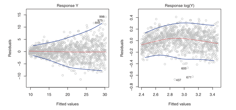
Figure 2: Left: the funnel shape indicates heteroscedasticity, Right: the response has been log transformed, and there is now no evidence of heteroscedasticity
Outliers
An outlier is a point from which \(y_i\) is far from the value predicted by the model. It is atypical for an outlier that does not have an unusual predictor value to have little effect on the least squares fit. However, it can cause other problems, such as dramatically altering the computed values of RSE, \(R^2\) and p-values.
Residual plots can clearly identify outliers. One solution is to simply remove the observation, but care must be taken to first identify whether the outlier is indicative of a deficiency with the model, such as a missing predictor.
High Leverage Points
Observations with high leverage have an unusual value for \(x_i\). High leverage observations typically have a substantial impact on the regression line. These are easy to identify, by looking for values outside the normal range of the observations. We can also compute the leverage statistic. for a simple linear regression:
\begin{equation} h_i = \frac{1}{n} + \frac{(x_i - \bar{x_i})^2}{\sum_{i’ = 1}^n(x_{i’} - \bar{x})^2} \end{equation}
Collinearity
Collinearity refers to the situation in which two or more predictor variables are closely related to one another. The presence of collinearity can pose problems in the regression context: it can be difficult to separate out the individual effects of collinear variables on the response. A contour plot of the RSS associated with different possible coefficient estimates can show collinearity.
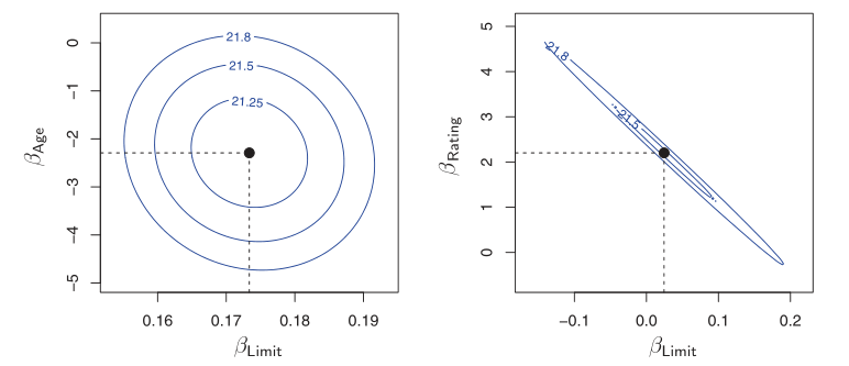
Figure 3: Left: the minimum value is well defined, Right: because of collinearity, there are many pairs \((\beta_{\text{Limit}}, \beta_{\text{Rating}})\) with a similar value for RSS
Another way to detect collinearity is to look at the correlation matrix of the predictors. An element of this matrix that is large in absolute value indicates a pair of highly correlated variables, and therefore a collinearity problem in the data.
Not all collinearity problems can be detected by inspection of the correlation matrix: it is possible for collinearity to exist between three or more variables even if no pairs of variables has a particularly high correlation. This situation is called multicollinearity. We instead compute the variance inflation factor (VIF). The VIF is the ratio of the variance of \(\hat{\beta_j}\) when fitting the full model divided by the variance of \(\hat{\beta_j}\) if fit on its own. The smallest possible value for VIF is 1, indicating a complete absence of collinearity. As a rule of thumb, a VIF exceeding values of 5 or 10 indicates a problematic amount of collinearity.
\begin{equation} \label{eqn:dfn:vif} \mathrm{VIF}(\hat{\beta_j}) = \frac{1}{1-R^2_{X_j|X_{-j}}} \end{equation}
where \(R^2_{X_j|X_{-j}}\) is the regression of \(X_j\) onto all of the other predictors.
The data consists of \(n\) observations on a dependent or response variable \(Y\), and \(p\) predictor or explanatory variables. The relationship between \(Y\) and \(X_1, X_2, \dots, X_p\) is represented by:
Linear Basis Function Models
We can extend the class of models by considering linear combinations of fixed non-linear functions of the input variables, of the form:
\begin{equation} y(\mathbf{x}, \mathbf{w}) = w_0 + \sum_{j=1}^{M-1} w_j \phi_j(\mathbf{x}) = \mathbf{w}^T\mathbf{\phi}(\mathbf{x}) \end{equation}
There are many choices on non-linear basis functions, such as the Gaussian basis function:
\begin{equation} \phi_j(x) = \mathrm{exp}\left\{ - \frac{(x - \mu_j)^2}{2s^2} \right\} \end{equation}
or the sigmoidal basis function:
\begin{equation} \phi_j(x) = \sigma\left( \frac{x - \mu_j}{s} \right) \end{equation}
Regression Diagnostics
In fitting a model to a given body of data, we would like to ensure that the fit is not overly determined by one or a few observations. The distribution theory, confidence intervals, and tests of hypotheses are valid and have meaning only if the standard regression assumptions are satisfied.
The Standard Regression Assumptions
Assumptions about the form of the model: The model that relates the response \(Y\) to the predictors \(X_1, X_2, \dots, X_p\) is assumed to be linear in the regression parameters \(\beta_0, \beta_1, \dots, \beta_p\) respectively:
\begin{equation} Y = \beta_0 + \beta_1X_1 + \dots + \beta_pX_p + \epsilon \end{equation}
which implies that the ith observation can be written as:
\begin{equation} y_{i} = \beta_0 + \beta_1x_{i1} + \dots \beta_px_{ip} + \epsilon_i, i = 1,2,\dots,n \end{equation}
Checking the linearity assumption can be done by examining the scatter plot of \(Y\) versus \(X\), but linearity in multiple regression is more difficult due to the high dimensionality of the data. In some cases, data transformations can lead to linearity.
Assumptions about the errors: The errors \(\epsilon_1, \epsilon_2, \dots, \epsilon_n\) are assumed to be independently and identically distributed normal random variables each with mean zero and a common variance \(\sigma^2\). Four assumptions are made here:
-
The error \(\epsilon_i\) has a normal distribution. This normality assumption can be validated by examining appropriate graphs of the residuals.
-
The errors \(\epsilon_i\) have mean 0.
-
The errors \(\epsilon_i\) have the same (but unknown) variance \(\sigma^2\). This is the constant variance assumption, also known as the homogeneity or homoscedasticity assumption. When this assumption does not hold, the problem is called the heterogeneity or the heteroscedasticity problem.
-
The errors \(\epsilon_i\) are independent of each other. When this assumption doesn’t hold, we have the auto-correlation problem.
Assumption about the predictors: Three assumptions are made here:
-
The predictor variables \(X_1, X_2, \dots, X_p\) are nonrandom. This assumption is satisfied only when the experimenter can set the values of the predictor variables at predetermined levels. When the predictor variables are random variables, all inferences are conditional, conditioned on the observed data.
-
The values \(x_{1j}, x_{2j}, \dots, x_{nj}\) are measured without error. This assumption is hardly ever satisfied, and errors in measurement will affect the residual variance, the multiple correlation coefficient, and the individual estimates of the regression coefficients. Correction for measurement errors of the estimated regression coefficients, even in the simplest case where all measurement errors are uncorrelated, requires a knowledge of the ratio between the variances and the random error. These quantities are seldom known.
-
The predictor variables \(X_1, X_2, \dots, X_p\) are assumed to be linearly independent of each other. This assumption is required to guarantee the uniqueness of the least squares solution. If this assumption is violated, the problem is referred to as the collinearity problem.
Assumption about the observations: All observations are equally reliable and have an approximately equal role in determining the regression results.
A feature of the method of least squares is that minor violations of the underlying assumptions do not invalidate the inferences or conclusions drawn from the analysis in a major way. However, gross violations can severely distort conclusions.
Types of Residuals
A simple method for detecting model deficiencies in regression analysis is the examination of residual plots. Residual plots will point to serious violations in one or more of the standard assumptions when they exist. The analysis of residuals may lead to suggestions of structure or point to information in the data that might be missed or overlooked if the analysis is based only on summary statistics.
When fitting the linear model to a set of data by least squares, we obtain the fitted values:
\begin{equation} \hat{y}_i = \hat{\beta}_0 + \hat{\beta}1 x_{i1} +\dots + \hat{\beta}_p x_{ip} \end{equation}
and the corresponding ordinary least squares residuals:
\begin{equation} e_i = y_i - \hat{y}_i \end{equation}
The fitted values can also be written in an alternative form as:
\begin{equation} \hat{y_i} = p_{i1}y_1 + p_{i2}y_2 + \dots + p_{in}y_n \end{equation}
where the \(p_{ij}\) are quantities that depend only on the values of the predictor variables. In simple regression \(p_{ij}\) is given by:
\begin{equation} p_{ij} = \frac{1}{n} + \frac{\left( x_i + \overline{x} \right) \left( x_j - \overline{x} \right)}{\sum (x_i - \overline{x})^2} \end{equation}
In multiple regression the \(p_{ij}\) are elements of matrix known as the hat or projection matrix.
The value \(p_{ii}\) is called the leverage value for the ith observation, because \(\hat{y}_i\) is a weighted sum of all the observations in \(Y\) and \(p_{ii}\) is the weight (leverage) given to \(y_i\) in determining the ith fitted value \(\hat{y}_i\). Thus, we have \(n\) leverage values, and they are denoted by:
\begin{equation} p_{11}, p_{22}, \dots, p_{nn} \end{equation}
When the standard assumptions hold, the ordinary residuals, \(e_1, e_2, \dots, e_n\) will sum to zero, but they will not have the same variance because:
\begin{equation} \textrm{Var}(e_i) = \sigma^2\left( 1 - p_{ii} \right) \end{equation}
To over come the problem of unequal variances, we standardize the ith residual \(e_i\) by dividing by its standard deviation:
\begin{equation} z_i = \frac{e_i}{\sigma \sqrt{1 - p_{ii}}} \end{equation}
This is called the ith standardized residual because it has mean zero and standard deviation 1. The standardized residuals depend on \(\sigma\), the unknown standard deviation of \(\epsilon\). An unbiased of \(\sigma^2\) is given by:
\begin{equation} \hat{\sigma}^2 = \frac{\sum e_i^2}{n - p - 1} = \frac{\sum (y_i - \hat{y}_i)^2}{n - p - 1} = \frac{\textrm{SSE}}{n -p-1} \end{equation}
An alternative unbiased estimate of \(\sigma^2\) is given by:
\begin{equation} \hat{\sigma}_{(i)}^2 = \frac{SSE_{(i)}}{n - p -2} \end{equation}
where \(SSE_{(i)}\) is the sum of squared residuals when we fit the model to the n - 1 observations by omitting the ith observation.
Using \(\hat{\sigma}\) as an estamite of \(\sigma\), we obtain:
\begin{equation} r_i = \frac{e_i}{\hat{\sigma}\sqrt{1 - p_{ii}}} \end{equation}
which we term the internally studentized residual. Using teh other unbiased estimate, we get:
\begin{equation} r_i^* = \frac{e_i}{\hat{\sigma_{(i)}}\sqrt{1 - p_{ii}}} \end{equation}
which is a monotonic transformation of \(r_i\). This is termed the externally studentized residual. The standardized residuals do not sum to zero, but they all have the same variance.
The externally standardized residuals follow a t-distribution with n - p - 2 degrees of freedom, but the internally standardized residuals do not. However, with a moderately large sample, these residuals should approximately have a standard normal distribution. The residuals are not strictly independently distributed, but with a large number of observations, the lack of independence may be ignored.
Graphical methods
Before fitting the model
Graphs plotted before fitting the model serve as exploratory tools. There are four categories of graphs:
1. One-dimensional graphs
One-dimensional graphs give a general idea of the distribution of each individual variable. One of the following graphs may be used:
- histogram
- stem-and-leaf display
- dot-plot
- box-plot
These graphs indicate whether the variable is symmetric, or skewed. When a variable is skewed, it should be transformed, generally using a logarithmic transformation. Univariate graphs also point out the presence of outliers in the variables. However, no observations should be deleted at this stage.
2. Two-dimensional graphs
We can take the variables in pairs and look at the scatter plots of each variable versus each other variable in the data set. These explore relationships between each pair of variables and identify general patterns. These pairwise plots can be arranged in a matrix format, known as the draftsman’s plot or the plot matrix. In simple regression, we expect the plot of \(Y\) versus \(X\) to show a linear pattern. However, scatter plots of \(Y\) versus each predictor variable may or may not show linear patterns.
Beyond these, there are rotation plots and dynamic graphs which serve as powerful visualizations of the data in more than 2 dimensions.
Graphs after fitting a model
The graphs after fitting a model help check the assumptions and assess the adequacy of the fit of a given model.
- Graphs checking linearity and normality assumptions
When the number of variables is small, the assumption of linearity can be checked by interactively and dynamically manipulating plots discussed in the previous section. However, this quickly becomes difficult with many predictor variables. Plotting the standardized residuals can help check the linearity and normality assumptions.
-
Normal probability plot of the standardized residuals: This is a plot of the ordered standardized residuals versus the normal scores. The normal scores are what we would expect to obtain if we take a sample of size \(n\) from a standard normal distribution. If the residuals are normally distributed, the ordered residuals should be approximately the same as the ordered normal scores. Under the normality assumption, this plot should resemble a straight line with intercept zero and slope of 1.
-
Scatter plots of the standardized residual against each of the predictor variables: Under the standard assumptions, the standardized residuals are uncorrelated with each of the predictor variables. If the assumptions hold, the plot should be a random scatter of points.
-
Scatter plot of the standardized residual versus the fitted values: Under the standard assumptions, the standardized residuals are also uncorrelated with the fitted values. Hence, this plot should also be a random scatter of points.
-
Index plot of the standardized residuals: we display the standardized residuals versus the observation number. If the order in which the observations were taken is immaterial, this plot is not needed. However, if the order is important, a plot of the residuals in serial order may be used to check the assumption of the independence of the errors.
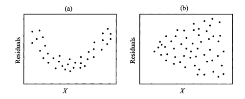
Figure 4: Scatter plots of residuals: (a) shows nonlinearity, and (b) shows heterogeneity
References
, Chatterjee and Hadi, n.d., @james2013introduction