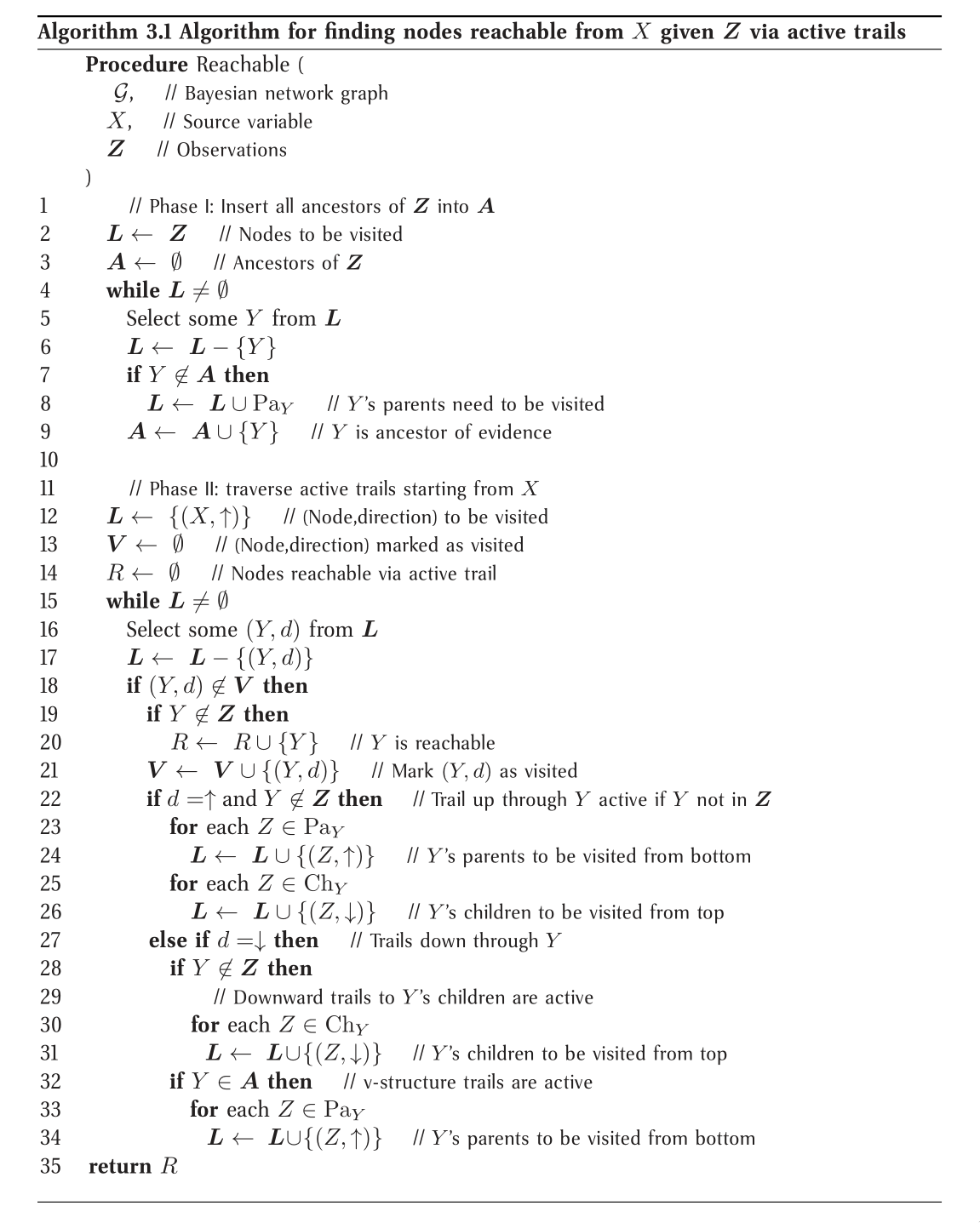
Probabilistic Graph Models
Motivation
Most tasks require a person or an automated system to reason: to take the available information and reach conclusions, both about what might be true in the world and about how to act. Probabilistic graphical models represent a general framework that can be used to allow a computer system to reason.
Using this approach of declarative representation, we construct, within the computer, a model of the system about which we would like to reason. This model encodes our knowledge of how the system works in a computer-readable form. This representation can then be manipulated by various algorithms that can answer questions based on the model.
The key property of a declarative representation is the separation of knowledge and reasoning. The representation has its own clear semantics, separate from the algorithms that one can apply to it. Thus, we can develop a general suite of algorithms that apply any model within a broad class, whether in the domain of medical diagnosis or speech recognition. Conversely, we can improve our model for a specific application domain without having to modify our reasoning algorithms constantly.
Uncertainty is a fundamental quantity in many real-world situations. To obtain meaningful conclusions, we need to reason not just about what is possible, but what is probable.
The calculus of probability theory provides us with a formal framework for considering multiple outcomes and their likelihood. This frameworks allows us to consider options that are unlikely, yet not impossible, without reducing our conclusions to content-free lists of every possibility.
One finds that probabilistic models are very liberating. Where in a more rigid formalism, we might find it necessary to enumerate every possibility, here we can often sweep a multitude of annoying exceptions and special cases under the probabilistic rug, by introducing outcomes that roughly correspond to “something unusual happens”. This type of approximation is often inevitable, as we can only rarely provide a deterministic specification of the behaviour of a complex system. Probabilistic models allow us to make this explicit, and therefore provide a model that is more faithful to reality.
Graphical Representation
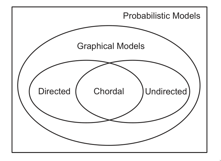
Probabilistic graphical models use a graph-based representation as the basis for compactly encoding a complex distribution over a high-dimensional space. In this graphical representation, the nodes correspond to the variables in our domain, and the edges correspond to direct probabilistic interactions between them.
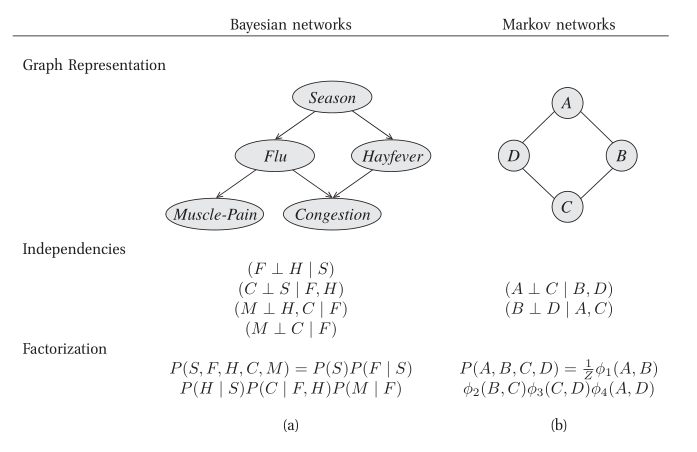
Figure 1: Different perspectives on probabilistic graphical models
Bayesian Networks
The goal is to represent a joint distribution \(P\) over some set of random variables \(\left\{X_1, \dots, X_n\right\}\). Even in the simplest case where these numbers are binary-valued, a joint distribution requires the specification of \(2^n-1\) numbers. For all but the smallest \(n\), the joint distribution in unmanageable from every perspective. Computationally, it is expensive to manipulate and generally too large to store in memory. Cognitively, it is impossible to acquire so many numbers from a human expect, moreover, the numbers are very small and do not correspond to events that people can reasonably contemplate. Statistically, if we want to learn the distribution from data, we would need ridiculously large amounts of data to estimate many parameters robustly. These problems have been the main barrier to the adoption of probabilistic methods for expert systems until the development of the methodologies presented below.
The compact representations explored are based on two key ideas: the representation of independence properties of the distribution, and the use of an alternative parameterization that allows us to exploit these fine-grained independencies.
Bayesian networks build on the same intuitions as the naive Bayes model by exploiting conditional independence properties of the distribution in order to allow a compact and natural representation. The core of the Bayesian network representation is the directed graph \(G = (V,E)\) together with a random variable \(x_i\) for each node \(i \in V\), one conditional probability distribution (CPD) p(x_i | xA_i) per node, specifying the probability of \(x_i\) conditioned on its parent’s values.
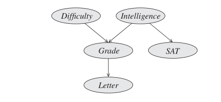
Figure 2: Example of a Bayesian Network graph
This graph \(G\) can be viewed in two very different ways:
- as a data structure that provides the skeleton for representing a joint distribution compactly in a factorized way;
- as a compact representation for a set of conditional independence assumptions about a distribution.
These two views, are in a strong sense, equivalent.
Bayesian Network Semantics
We can formally define the Bayesian network structure as follows:
Let \(\mathrm{Pa}_{X_i}^G\) denote the parents of \(X_i\) in G, and \(\mathrm{NonDescendants}_{X_i}\) denote the variables in the graph that are not descendants of \(X_i\). Then \(G\) encodes the following set of independence assumptions, called the local independencies, denoted by \(I_l(G)\):
\begin{equation} \text{ For each variable } X_i: \left( X_i \perp \mathrm{NonDescendants}_{X_i} | \mathrm{Pa}_{X_i}^G \right) \end{equation}
In other words, the local independencies state that each node \(X_i\) is conditionally independent of its nondescendants given its parents.
The formal semantics of a Bayesian network graph is as a set of independence assertions. On the other hand, our representation was a graph annotated with conditional probability distributions (CPDs). Here, we show that these two definitions are, in fact equivalent. A distribution \(P\) satisfies the local independencies associated with a graph \(G\) if and only if \(P\) is representable as a set of CPDs associated with the graph \(G\). We begin by formalizing the basic concepts.
I-Maps
Let \(P\) be a distribution over \(\mathcal{X}\). We define \(\mathcal{I}(P)\) to be the set of independence assertions of the form \((X \perp Y | Z)\) that hold in \(P\).
Now, we need to show that \(\mathcal{I}_l(G) \subseteq \mathcal{I}(P)\).
Let \(K\) be any graph object associated with a set of independencies \(\mathcal{I}(K)\). We say that \(K\) is an I-map for a set of independencies \(\mathcal{I}\) if \(\mathcal{I}(K) \subseteq \mathcal{I}\).
Now, we can say we need to show that \(G\) is an I-map for \(P\).
For \(G\) to be an I-map for \(P\), it is necessary that \(G\) does not mislead us regarding independencies of \(P\): any independence that \(G\) asserts must also hold in \(P\). Conversely, \(P\) may have additional independencies not reflected in \(G\).
I-Map to Factorization
A BN structure \(G\) encodes a set of conditional independence assumptions; every distribution for which \(G\) is an I-map must satisfy these assumptions.
Consider the joint distribution \(P(I, D, G, L, S)\); from the chain rule for probability, we can decompose the distribution in the following way:
\begin{equation} P(I, D, G, L, S) = P(I) P(D|I) P(G|I, D) P(L | I, D, G) P(S | I, D, G, L) \end{equation}
This decomposition requires no assumptions. We may however be able to apply our conditional independence assumptions induced from the BN.
We say that a distribution \(P\) over the same space factorizes according to a BN graph \(G\) if \(P\) can be expressed as a product:
\begin{equation} P(X_1, \dots, X_n) = \prod_{i=1}^{n} P(X_i | \mathrm{Pa}_{X_i}^G). \end{equation}
This equation is called the chain rule for BNs. The individual factors \(P(X_i | \mathrm{Pa}_{X_i}^G)\) are called conditional probability distributions (CPDs) or local probabilistic models.
We can now show that if \(G\) is a BN structure over a set of random variables \(X\), and \(P\) be a joint distribution over the same space, then if \(G\) is an I-map for \(P\), \(P\) factorizes according to \(G\).
Proof:
Assume, without loss of generality, that \(X_1, \dots, X_n\) is a topological ordering of the variables in \(X\) relative to \(G\). First, we use the chain rule for probabilities:
\begin{equation} P(X_1, \dots, X_n) = \prod_{i=1}^{n}P(X_i | X_1, \dots, X_{i-1}). \end{equation}
Now consider one of the factors \(P(X_i|X_1, \dots, X_{i-1})\). As \(G\) is an I-map for \(P\), we have \((X_i \perp \mathrm{ND}_{X_i} | \mathrm{Pa}_{X_i}^G) \in I(P)\). By assumption, all of \(X_i\)‘s parents are in the set \(X_1, \dots, X_{i-1}\). Furthermore, none of \(X_i\)‘s descendants can possibly be in the set. Hence
\begin{equation} \left\{ X_1, \dots, X_{i-1} \right\} = \mathrm{Pa}_{X_i} \in \mathbf{Z} \end{equation}
where \(\mathbf{Z} \in \mathrm{ND}_{X_i}\). Form the local independencies for \(X_i\) and from the position property it follows that \(X_i \perp \mathbf{Z} | \mathrm{Pa}_{X_i}\). Hence \(P(X_i| X_1, \dots X_{i-1}) = P(X_i | \mathrm{Pa}_{X_i})\).
Applying this transformation to all of the factors in the chain rule decomposition gives the desired result.
Factorization to I-map
This is simple to prove, by manipulation of probabilities.
Independencies in Graphs
Dependencies and independencies are crucial for understanding the behaviour of a distribution. Independency properties are also important for answering queries: they can be exploited to reduce substantially the computational cost of inference. Therefore, it is important that our representations make these properties clearly visible both to a user and to algorithms that manipulate the BN data structure.
The immediate question that arises is whether there exist independence properties that we can read off directly from \(G\).
D-separation
We want to be able to guarantee that an independence \((\mathbf{X} \perp \mathbf{Y} | \mathbf{Z})\), holds in a distribution associated with a BN structure \(G\). It helps to consider its converse: “Can we imagine a case where it does not?”
Direct Connection
If \(X \rightarrow Y\), then we can construct a distribution such that \(X\) and \(Y\) are correlated regardless of any evidence about of the other variables in the network. (e.g. \(Val(X) = Val(Y)\))
Indirect Connection
Consider a 3-node network where \(X\) and \(Z\) are not directly connected but through \(Y\). There are four possible 2-edge trails:
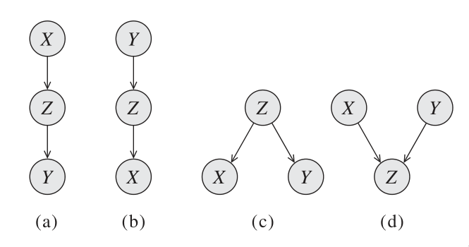
We say that Q, W are d-separated when variables \(O\) are observed if they are not connected by an active path. An undirected path in the Bayesian network \(G\) is called active given observed variables \(O\) if for every triple of variables \(X, Y, Z\) on the path, one of the following holds:
- Casual trail
- \(X \leftarrow Y \leftarrow Z, Y \not\in O\) active iff \(Y\) is not observed
- Evidential trail
- \(X \rightarrow Y \rightarrow Z, Y \not\in O\) active iff \(Y\) is not observed
- Common cause
- \(X \leftarrow Y \rightarrow Z, Y \not\in O\) active iff \(Y\) is not observed
- Common effect
- \(X \rightarrow Y \leftarrow Z, Y \text{ or any descendants} \in O\) active iff either \(Y\) or one of \(Y\)‘s descendants is observed
Consider the general trail \(X_1 \rightleftharpoons X_2 \rightleftharpoons \dots \rightleftharpoons X_n\). Let \(\mathbf{Z}\) be a subset of observed variables. Then the trail is active given \(\mathbf{Z}\) if:
- Whenever we have a v-structure \(X_{i-1} \rightarrow X_i \leftarrow X_{i+1}\), then \(X_i\) or one of its descendants are in \(\mathbf{Z}\);
- no other node along the trail is in \(\mathbf{Z}\).
Let \(\mathbf{X}, \mathbf{Y}, \mathbf{Z}\) be three sets of nodes in \(\mathcal{G}\). We say that \(\mathbf{X}\) and \(\mathbf{Y}\) are d-separated given \(\mathbf{Z}\), denoted \(\mathrm{d-sep}_{\mathcal{G}}(\mathbf{X}; \mathbf{Y} | \mathbf{Z})\), if there is no active trail between any node \(X \in \mathbf{X}\), and \(Y \in \mathbf{Y}\) given \(\mathbf{Z}\). We use \(\mathcal{I}(\mathcal{G})\) to denote this set of independencies that correspond to d-separation:
\begin{equation} \mathcal{I}(\mathcal{G}) = \left\{ (\mathbf{X} \perp \mathbf{Y} | \mathbf{Z}) : \mathrm{d-sep}_{\mathcal{G}}(\mathbf{X}; \mathbf{Y} | \mathbf{Z}) \right\} \end{equation}
This set is also called the set of global Markov independencies. These independencies are precisely those that are guaranteed to hold for every distribution over \(G\).
A nice tutorial on d-separation can be found here.
Markov Blanket
Consider a joint distribution \(p(X_1, \dots, x_D)\) represented by a directed graph having \(D\) nodes. Consider the conditional distribution of a particular node with variables \(x_i\) conditioned on all the remaining variables \(x_{j \ne i}\). We have:
\begin{equation} p(x_i | x_{\{j \ne i\}}) = \frac{p(x_1, \dots, x_D)}{\int p(x_1, \dots, x_D) dx_i} = \frac{\prod_{k}p(x_k | \textrm{pa}_k)}{\prod_k p(x_k | \textrm{pa}_k)dx_i} \end{equation}
We observe that any factor \(p(x_k | \textrm{pa}_k)\) that does not have any functional dependence on \(x_i\) can be taken outside the integral, and will therefore cancel between the numerator and the denominator. The only factors that will remain are the conditional distribution \(p(x_i | \textrm{pa}_i)\) for the node \(x_i\) itself, and conditional distributions for any nodes \(x_k\) such that node \(x_i\) is in teh conditioning set of \(p(x_k | \textrm{pa}_k)\), in other words for which \(x_i\) is a parent of \(x_k\). The conditional \(p(x_i | \textrm{pa}_i)\) will depend on the parents of node \(x_i\), and the conditionals \(p(x_k | \textrm{pa}_k)\) will depend on nthe children of \(x_i\), as well as the co-parents: variables corresponding to parents of node \(x_k\) other than \(x_i\). This set of nodes is called the Markov Blanket.
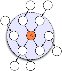
Figure 3: An illustration of the Markov Blanket. (Source)
Soundness and Completeness
- Soundness
- If a distribution \(P\) factorizes according to \(G\), then \(\mathcal{I}(G) \subseteq \mathcal{I}(P)\).
- Completeness
- If we have 2 variables \(X\) and \(Y\) that are independent given \(\mathbf{Z}\), then \(X\) and \(Y\) are d-separated. We find that this is ill-defined, because it does not specify the distribution in which \(X\) and \(Y\) are independent.
- Faithful
- A distribution \(P\) is faithful to \(G\) if, whenever \((X \perp Y | \mathbf{Z}) \in I(P)\), then \(\mathrm{d-sep}_{G}(X;Y|\mathbf{Z})\). Any independence in \(P\) is reflected in the d-separation properties of the graph.
The notion of faithfulness is the converse of our notion of soundness. However, it can be shown that this desirable property of faithfulness is false.
We can, however, adopt a weaker but useful definition of completeness:
If \((X \perp Y | \mathbf{Z})\) in all distributions \(P\) that factorize over \(G\), then \(\mathrm{d-sep}_G(X;Y|\mathbf{Z})\).
Using this definition, we can show that If \(X\) and \(Y\) are not d-separated given \(\mathbf{Z}\) in \(G\), then \(X\) and \(Y\) are dependent given \(Z\) in some distribution \(P\) that factorizes over \(G\).
This completeness result tells us that our definition of \(I(G)\) is the maximal one: for any independence assertion that is not a consequence of d-separation in \(g\), we can always find a counterexample distribution \(P\) that factorizes over \(G\).
In fact, for almost all distributions \(P\) that factorize over \(G\), that is for all distributions except for a set of measure zero in the space of CPD parameterizations, we have \(I(P) = I(G)\).
An algorithm for d-separation
There is a linear-time (in the size of the graph) algorithm for determining the set of d-separations. The algorithm has 2 phases:
- Traverse the graph bottom up, from the leaves to the roots, marking all nodes that are in \(\mathbf{Z}\) or that have descendants in \(\mathbf{Z}\). These nodes will serve to enable v-structures.
- Traverse breadth-first from \(X\) to \(Y\), stopping the traversal along a trail when we get to a blocked node.
A node is blocked if:
- it is the “middle” node in a v-structure and unmarked in phase I, or
- It is not a middle node and is in \(\mathbf{Z}\)
If the BFS gets us from \(X\) to \(Y\), then there is an active trail between them.
I-equivalence
The notion of \(I(G)\) specifies a set of conditional independence assertions that are associated with a graph. This allows us to abstract away of details of the graph structure, viewing it purely as a specification of independence properties.
One important implication of this perspective is the observation that very different BN structures can actually be equivalent, in that they encode the same set of conditional independence assumptions.
This brings us to the notion of I-equivalence:
Two graphs \(K_1\) and \(K_2\) over \(X\) are I-equivalent if \(I(K_1) = I(K_2)\). The set of all graphs over \(X\) are partitioned into mutually exclusive and exhaustive I-equivalence classes.
This notion implies that any distribution \(P\) that can be factorized over one of these graphs can be factorized over the other. Furthermore, there is no intrinsic property of \(P\) that would allow us to associate it with one graph rather than an equivalent one. This observation has important implications with respect to our ability to determine the directionality of influence.
From Distributions to Graphs
Given a distribution \(P\), to what extent can we construct a graph \(G\) whose independencies are a reasonable surrogate for the independencies in \(P\)? We will never actually take a fully-specified distribution \(p\) and construct a graph \(G\) for it, as this is way too large. However, answering this question is an important contextual exercise, that h helps in understanding the process of constructing a BN that represents our model of the world.
Minimal I-maps
One approach to finding a graph that represents a distribution \(p\) is simply to take any graph that is an I-map for \(P\). However, a complete graph is an I-map for any distribution, but it does not reveal any independencies in the distribution. This intuition leads us to the definition of a minimal I-map:
A graph \(K\) is a minimal I-map for a set of independencies \(i\) if it is an I-map for \(I\), and if the removal of even a single edge from \(K\) renders it not an I-map.
To obtain a minimal I-map we simply follow a natural algorithm that arises through the factorization theorem. Note that the minimal I-map is not necessarily unique in this construction.
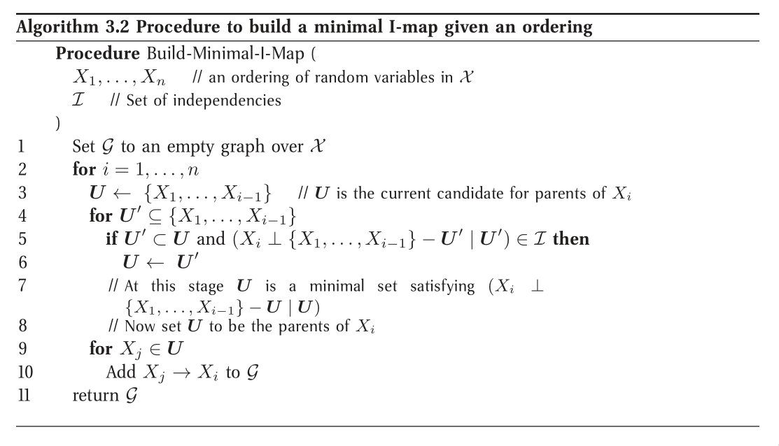
Minimal I-maps fail to capture all the independencies that hold in the distribution. Hence, that \(G\) is a minimal I-map for \(P\) is far from a guarantee that \(G\) captures the independence structure in \(P\).
Perfect Maps
A graph \(K\) is a P-map for a distribution \(P\), for a set of independencies \(I\) if we have that \(I(K) = I\). We say that \(K\) is a perfect map for \(P\) if \(I(K) = I(P)\).
Unfortunately, not every distribution has a perfect map. There exists an algorithm for finding the DAG representing the P-map for a distribution of a P-map if it exists, but is quite involved. See Koller, Friedman, and Bach, n.d..
Undirected Graphical Models
(The bulk of the material is from Murphy’s book Murphy, n.d.)
For some domains, being forced to choose a direction for the edges, as required by a DGM is awkward. For example, if we’re modelling an image, we might suppose that the neighbouring pixels are correlated. We may form a DAG model with a 2d lattice topology as such:
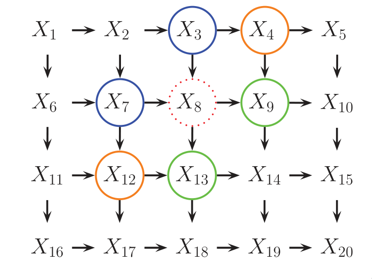
Figure 4: 2d lattice represented as a DAG.
However, representing the conditional probabilities in this way is rather unnatural: the Markov blanket of node \(X_8\) includes its non-neighbours. Instead, we may want to use a UGM, or Markov Random Field (MRF).
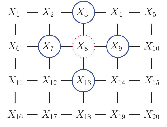
Figure 5: UGM representation of the lattice topology.
Conditional Independence Properties of UGMs
UGMs define CI relationships via simple graph separation as follows:
- global Markov property
- \(A \perp B | \mathbf{C}\) if there is no path between A and B in the graph upon removing all nodes in \(\mathbf{C}\).
- local Markov property
- \(A \perp V \setminus \{\textrm{mb}(A), A\} | \textrm{mb}(A)\)
- pairwise Markov property
- \(A \perp B | V \setminus \left{ A, B\right}\)
The global Markov property implies the local and pairwise Markov properties. If \(p(x) > 0\) for all \(x\), then the pairwise Markov property implies the global Markov property. This result allows us to use pairwise CI statements to construct a graph from which global statements can be extracted.
Representation Power
DGMs and UGMs can perfectly represent different set of distributions. The set of distributions that are perfectly represented by both DGMs and UGMs are termed chordal.
In general, CI properties in UGMs are monotonic, in the following sense: if \(A \perp B | C\), then \(A \perp B | C \cup D\). In DGMs, CI properties can be non-monotonic, since conditioning on extra variables can eliminate conditional independencies due to explaining away.
If all the variables are collapsed in each maximal clique to make “mega-variables”, the resulting graph will be a tree if the distribution is chordal.
The Undirected alternative to d-separation
It is tempting tot simply convert the DGM to a UGM by dropping the orientation of the edges, but this is incorrect because a v-structure has different CI properties than the undirected chain. To avoid such incorrect CI statemnets, we can add edges between the “unmarreid” parents A and C, and then drop the arrows from the edges, forming in a connected undirected graph. This process is called moralization.
Moralization loses some CI information, and therefore we cannot used a moralized UGM to determine CI properties of the DGM.
Parameterization of MRFs
Since there is no topological ordering in an unordered graph, \(p(y)\) cannot be represented with the chain rule. Instead, potential functions or factors are associated with each maximal clique in the graph The join distribution is defined to be proportional to the product of clique potentials. The Hammersley-Clifford theorem shows that any positive distribution whose CI properties can be represented by a UGM can be represented in this way.
A positive distribution \(p(y) > 0\) satisfies the CI properties of an undirected graph \(G\) iff p can be represented as a product of factors, one per maximal clique, i.e.,
\begin{equation} p(\mathbf{y}|\mathbf{\theta}) = \frac{1}{Z(\mathbf{\theta})} \prod_{c\in \mathcal{C}} \Phi_c(\mathbf{y}_c | \mathbf{\theta}_c) \end{equation}
were \(C\) is the set of all the (maximal) cliques of \(G\), and \(Z(\mathbf{\theta})\) is the partition function given by
\begin{equation} Z(\mathbf{\theta}) = \sum_{x} \prod_{c \in \mathcal{C}} \Phi_c(\mathbf{y}_c|\mathbf{\theta}_c) \end{equation}
Connection between statistical physics
There is a model known as the Gibbs distribution, which can be written as follows:
\begin{equation} p(\mathbf{y} | \mathbf{\theta}) = \frac{1}{Z(\mathbf{\theta})} \mathrm{exp} \left( - \sum_{c} E(\mathbf{y}_c | \mathbf{\theta}_c) \right) \end{equation}
where \(E(\mathbf{y}_c)\) is the energy associated with the variables in clique \(c\). We can convert this to a UGM by defining:
\begin{equation} \Phi_c(\mathbf{y}_c | \mathbf{\theta}_c) = \mathrm{exp}\left( - E(\mathbf{y}_c | \mathbf{\theta}_c) \right) \end{equation}
Here we see that high probability states correspond to low energy configurations. We are also free to restrict the parameterization to the edges of the graph. A rather convenient formulation is the pairwise MRF.
Representing Potential Functions
If the variables are discrete, we can represent the potential or energy functions as tables of (non-negative) numbers, as with CPTs. However, the potentials are not probabilities, but rather a representation of relative “compatibility” or “happiness” between the different assignments.
A more general approach is to define the log potentials as a linear function of the parameters:
\begin{equation} \log \psi_c (\mathbf{y}_c) = \phi_c (\mathbf{y}_c)^T \mathbf{\theta}_c \end{equation}
where \(\phi_c (\mathbf{x}_c_)\) a feature vector derived from the values of the variables \(mathbf{y}_c\). The resultant log probability has the form:
\begin{equation} \log p(\mathbf{y} | \mathbf{\theta}) = \sum_{c} \phi_c(\mathbf{y}_c)^T \mathbf{\theta}_c - Z(\mathbf{\theta}) \end{equation}
This is also known as the maximum entropy or log linear model.
Several popular probability models, such as the Ising model, Potts model and Hopfield networks, can be conveniently expressed as UGMs.
Parameter Estimation in UGMs
Consider an MRF in log-linear form:
\begin{equation} p(\mathbf{y} | \mathbf{\theta}) = \frac{1}{Z(\mathbf{\theta})} \mathrm{exp} \left( \sum_{c}\mathbf{\theta_c}^T \phi_c(\mathbf{y})\right) \end{equation}
where \(c\) indexes the cliques. The scaled log-likelihood is given by:
\begin{equation} l(\mathbf{\theta}) = \frac{1}{N}\sum_{i}\log(\mathbf{y}_i|\mathbf{\theta}) = \frac{1}{N}\sum_{i}\left[ \sum_{c}\mathbf{\theta}_c^T\phi_c(\mathbf{y}_i) - \log Z(\mathbf{\theta}) \right] \end{equation}
Since MRFs are in the exponential family, we know that this function is convex in \(\mathbf{\theta}\), and has a unique global maximum which we can find using gradient-based optimizers.
The derivative for the weights of a particular clique is given by:
\begin{equation} \frac{\partial l}{\partial \mathbf{\theta}_c} = \frac{1}{N}\sum_{i}\left[ \phi_c(\mathbf{y}_i) - \frac{\partial}{\partial \mathbf{\theta}_c} \log Z(\mathbf{\theta}) \right] \end{equation}
The derivative of the log partition function wrt to \(\mathbf{\theta_c}\) is just the expectation of the cth feature under the model, and hence the gradient of the log-likelihood is:
\begin{equation} \frac{\partial l}{\partial \mathbf{\theta}_c} = \frac{1}{N}\sum_{i}\left[ \phi_c(\mathbf{y}_i) - \mathcal{E}[\phi_c(\mathbf{y})]\right] \end{equation}
In the first term, we fix \(\mathbf{y}\) to its observed values; this is sometimes called the clamped term. In the second term \(\mathbf{y}\) is free; this is sometimes called the unclamped term. Computing the unclamped term requires inference in the model, and must be done once per gradient step, making it much slower than DGM training.
Approximate methods for computing the MLEs of MRFs
When fitting a UGM there is (in general) no closed form solution for the ML or the MAP estimate of the parameters, so we need to use gradient-based optimizers. This gradient requires inference. In models where inference is intractable, learning is also intractable. This motivates computationally faster alternatives to ML/MAP estimation, such as pseudo likelihood, and stochastic maximum likelihood.
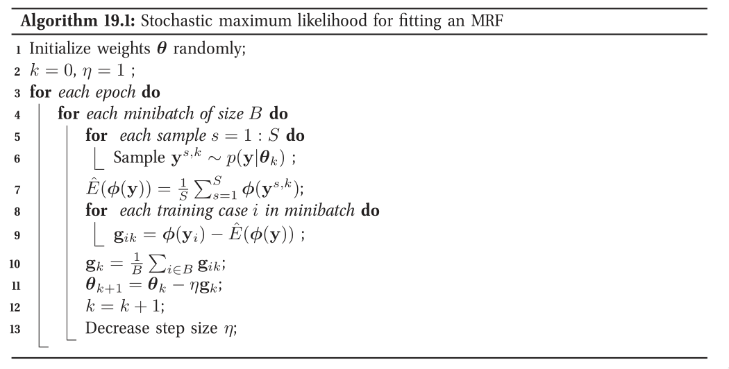
Figure 6: Stochastic maximum likelihood
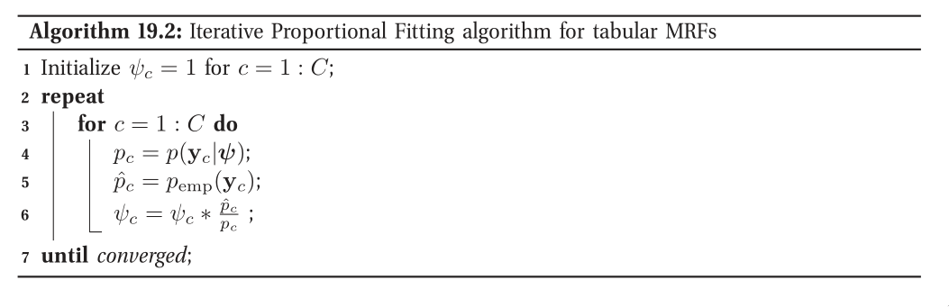
Figure 7: Iterative Proportional Fitting
Conditional Random Fields (CRFs)
A CRF is a version of an MRF where all the clique potentials are conditioned on input features:
\begin{equation} p(\mathbf{y} | \mathbf{x}, \mathbf{w}) = \frac{1}{Z(\mathbf{x}, \mathbf{w})} \prod_{c} \psi_c(\mathbf{y}_c | \mathbf{x}, \mathbf{w}) \end{equation}
It can be thought of as a structured output extension of logistic regression. A log-linear representation of the potentials is often assumed.
The advantage of a CRF over a MRF is analogous to the advantage of a discriminative classifier over a generative classifier, where we don’t need to “waste resources” modeling things that we always observe, but instead model the distribution of labels given the data.
In the CRF, we can also make the potentials of the model be data-dependent. For example, we can make the latent labels in an NLP problem depend on global properties of the sentence.
However, CRF requires labeled training data, and are slower to train.