Control As Inference
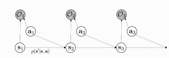
Figure 1: PGM for decision making for the first 3 time-steps
We introduce a binary variable for Optimality \(\mathcal{O}_t\) at each time-step. We want to infer: \(p(\tau | \mathcal{O}_{1:T})\)
If we choose \(p(O_t | s_t, a_t) = \mathrm{exp}(r(s_t, a_t))\), then:
\begin{align}
p(\tau | \mathcal{O}_{1:T}) &= \frac{p(\tau,
\mathcal{O}_{1:T})}{p(\mathcal{O}_{1:T})}
\\\
&\propto \prod_{t} \mathrm{exp}(r(s_t,
a_t)) \\\
&= p(\tau) \mathrm{exp} \left( \sum_{t}
r(s_t, a_t) \right)
\end{align}
With this Probabilistic Graph Model, we can:
- model sub-optimal behaviour (important for inverse RL)
- can apply inference algorithms to solve control and planning problems
- provides an explanation for why stochastic behaviour may be preferred (useful for exploration and transfer learning)
Inference
- compute backward messages \(\beta_t (s_t, a_t) = p(\mathcal{O}_{t:T} | s_t, a_t)\)
- compute policy \(p(a_t | s_t, \mathcal{O}_{1:T})\), the policy of this model under assumption of optimality
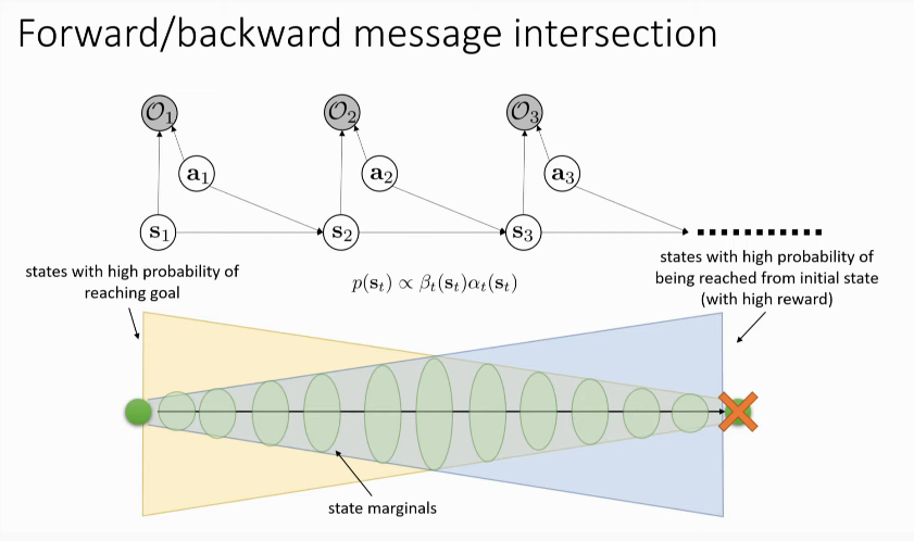
- compute forward messages \(\alpha_t(s_t) = p(s_t | \mathcal{O}_{1:t-1})\)
- useful for figuring out which states the optimal policy lands in, for the inverse RL problem (not used for forward RL)
Backward Messages
\begin{align}
\beta_t (s_t, a_t) &= p(\mathcal{O}_{t:T} | s_t, a_t) \\\
&= \int p(\mathcal{O}_{t:T}, s_{t+1} | s_t, a_t)
ds_{t+1} \\\
&= \int p(\mathcal{O}_{t+1:T}|s_{t+1})
p(s_{t+1}|s_t,a_t) p(\mathcal{O}_t | s_t, a_t)
ds_{t+1}
\end{align}
\begin{align}
p(\mathcal{O}_{t+1:T} | s_{t+1}) &= \int p(\mathcal{O}_{t+1:T} |
s_{t+1}, a_{t+1})p(a_{t+1}| s_{t+1}) da_{t+1} \\\
&= \int \beta_t(s_{t+1}, a_{t+1}) da_{t+1}
\end{align}
where we assume actions are likely a priori uniform. From these equations, we can get:
For \(t = T-1 \mathrm{ to } 1\):
\begin{equation} \beta_t(s_t, a_t) = p(\mathcal{O}_t | s_t, a_t) E_{s_{t+1} \sim p(s_{t+1},a_{t+1})} \left[ \beta_{t+1} (s_{t+1}) \right] \end{equation}
\begin{equation} \beta_{t}(s_t) = E_{a_t \sim p(a_t | s_t)} \left[ \beta_t(s_t, a_t) \right] \end{equation}
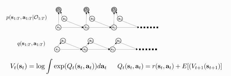
If we choose \(V_t (s_t) = \log \beta_t (s_t)\) and \(Q_t(s_t, a_t) = \log \beta_t (s_t, a_t)\):
\begin{align}
V_t(s_t) &= \log \int \mathrm{exp} (Q_t(s_t, a_t))da_t \\\
&\rightarrow \mathrm{max}_{a_t} Q_t(s_t, a_t) \textrm { as
} Q_t(s_t, a_t) \textrm { gets bigger }
\end{align}
For \(Q\):
\begin{equation} Q_t (s_t, a_t) = r(s_t, a_t) + \log E\left[ \mathrm{exp} (V_{t+1} (s_{t+1}, a_{t+1})) \right] \end{equation}
In a deterministic transition setting, the log and exp cancel out. However, this otherwise results in an optimistic transition, which is not a good idea!
What if the action prior is not uniform? We can always fold the action prior into the reward!
Policy computation
\begin{align}
p(a_t | s_t, \mathcal{O}_{1:T}) &= \pi (s_t | a_t) \\\
&= p(a_t | s_t, \mathcal{O}_{t:T})
\\\
&= \frac{\beta_t(s_t,
a_t)}{\beta_t(s_t)}p(s_t|a_t) \\\
&= \frac{\beta_t(s_t,
a_t)}{\beta_t(s_t)}
\end{align}
It turns out the policy is just the ratio between the 2 backward messages. Substituting \(V\) and \(Q\):
\begin{equation} \pi(a_t | s_t) = \mathrm{exp}(Q_t(s_t, a_t) - V_t(s_t)) = \mathrm{exp}(A_t(s_t, a_t)) \end{equation}
One can also add a temperature: \(\pi(a_t | s_t) = \mathrm{exp}(\frac{1}{\alpha} A_t(s_t, a_t))\)
Forward Messages
\begin{equation} p(s_t) \propto \beta_t(s_t) \alpha_t(s_t) \end{equation}
same derivations as Hidden Markov Model!
Resolving Optimism with Variational Inference
For more, see Levine, n.d..