Actor-Critic
Actor-Critic improves on Policy Gradients methods by introducing a critic.
Recall the objective:
\begin{equation} \nabla_{\theta} J(\theta) \approx \frac{1}{N} \sum_{i=1}^{N} \sum_{t=1}^{T} \nabla_{\theta} \log \pi_{\theta}\left(\mathbf{a}_{i, t} | \mathbf{s}_{i, t}\right) \hat{Q}_{i, t} \end{equation}
The question we want to address is: can we get a better estimate of the reward-to-go?
Originally, we were using the single-trajectory estimate of the reward-to-go. If we knew the true expected reward-to-go, then we would have a lower variance version of the policy gradient.
We define the advantage function as \(A^\pi(s_t,a_t) = Q^\pi(s_t, a_t) - V^\pi(s_t)\). \(V^\pi(s_t)\) can be used as baseline \(b\), and we obtain the objective:
\begin{equation} \nabla_{\theta} J(\theta) \approx \frac{1}{N} \sum_{i=1}^{N} \sum_{t=1}^{T} \nabla_{\theta} \log \pi_{\theta}\left(\mathbf{a}_{i, t} | \mathbf{s}_{i, t}\right) A^\pi(s_{i,t}, a_{i,t}) \end{equation}
Value Function Fitting
Recall:
\begin{array}{l}
{Q^{\pi}\left(\mathbf{s}_{t},
\mathbf{a}_{t}\right)=\sum_{t^{\prime}=t}^{T}
E_{\pi_{\theta}}\left[r\left(\mathbf{s}_{t^{\prime}},
\mathbf{a}_{t^{\prime}}\right) | \mathbf{s}_{t},
\mathbf{a}_{t}\right]} \\\
{V^{\pi}\left(\mathbf{s}_{t}\right)=E_{\mathbf{a}_{t} \sim
\pi_{\theta}\left(\mathbf{a}_{t} |
\mathbf{s}_{t}\right)}\left[Q^{\pi}\left(\mathbf{s}_{t},
\mathbf{a}_{t}\right)\right]} \\\
{A^{\pi}\left(\mathbf{s}_{t},
\mathbf{a}_{t}\right)=Q^{\pi}\left(\mathbf{s}_{t},
\mathbf{a}_{t}\right)-V^{\pi}\left(\mathbf{s}_{t}\right)} \\\
{\nabla_{\theta} J(\theta) \approx \frac{1}{N} \sum_{i=1}^{N}
\sum_{t=1}^{T} \nabla_{\theta} \log \pi_{\theta}\left(\mathbf{a}_{i,
t} | \mathbf{s}_{i, t}\right) A^{\pi}\left(\mathbf{s}_{i, t},
\mathbf{a}_{i, t}\right)}
\end{array}
We can choose to fit \(Q^{\pi}\), \(V^{\pi}\) or \(A^{\pi}\), each have their pros and cons.
We can write:
\begin{equation} Q^\pi (s_t, a_t) \approx r(s_t, a_t) + V^{\pi}(s_{t+1}) \end{equation}
\begin{equation} A^{\pi}(s_t, a_t) \approx r(s_t, a_t) + V^{\pi}(s_{t+1}) - V^{\pi}(s_t) \end{equation}
Classic actor-critic algorithms fit \(V^\pi\), and pay the cost of 1 time-step to get \(Q^\pi\).
We do Monte Carlo evaluation with function approximation, estimating \(V^\pi (s_t)\) as:
\begin{equation} V^\pi (s_t) \approx \sum_{t'=t}^{T}r(s_{t’}, a_{t’}) \end{equation}
Our training data consists of \(\left\{\left(s_{i,t}, \sum_{t'=t}^T r (s_{i,t’}, a_{i,t’})\right)\right\}\), and we can just fit a neural network with regression.
Alternatively, we can decompose the ideal target, and use the old \(V^\pi\):
\begin{equation} y_{i,t} = \sum_{t'=t}^{T} E_{\pi_{\theta}} [r(s_{t’}, a_t’) | s_{i,t}] \approx r(s_{i,t}, a_{i,t}) + \hat{V}_{\phi}^\pi(s_{i,t+1}) \end{equation}
This is a biased estimate, but might have much lower variance. This works when the policy does not change much and the previous value function is a decent estimate. Since it is using a the previous value function, it is also called a bootstrapped estimate.
Discount Factors
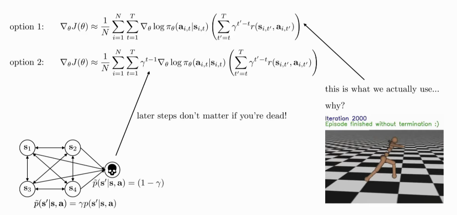
The problem with the bootstrapped estimate is that with long horizon problems, \(\hat{V}_\phi^\pi\) can get infinitely large. A simple trick is to use a discount factor:
\begin{equation} y_{i,t} \approx r(s_{i,t}, a_{i,t}) + \gamma \hat{V}_\phi^\pi(s_{i,t+1}) \end{equation}
where \(\gamma \in [0,1]\).
We can think of \(\gamma\) as changing the MDP, introducing a death state with reward 0, and the probability of transitioning to this death state is \(1 - \gamma\). This causes the agent to prefer better rewards now than later.
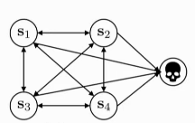
Figure 1: \(\gamma\) modified MDP
We can then modify \(\hat{A}^\pi\):
\begin{equation} \hat{A}^{\pi}(s_t, a_t) \approx r(s_t, a_t) + \gamma \hat{V}^{\pi}(s_{t+1}) - \hat{V}^{\pi}(s_t) \end{equation}
\(\gamma\) can be interpreted as a way to limit variance, and prevent the infinite sum (think about what happens when \(\gamma\) gets bigger).
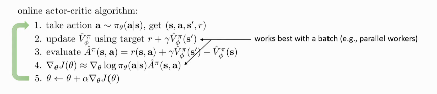
Algorithm
- sample \(\left\{s_i, a_i\right\}\) from \(\pi_{\theta}(a\s)\)
- Fit \(\hat{V}_\phi^{\pi}(s)\) to the sampled reward sums
- Evaluate \(\hat{A}^\pi(s_i, a_i) = r(s_i a_i) + \hat{V}_\phi^\pi(s_i’)-\hat{V}_\phi^\pi(s_i)\)
- \(\nabla_{\theta} J(\theta) \approx \sum_i \nabla_{\theta} \log \pi_{\theta}\left(\mathbf{a}_{i} | \mathbf{s}_{i}\right) \hat{A}^{\pi}\left(\mathbf{s}_{i}, \mathbf{a}_{i}\right)\)
- \(\theta \leftarrow \theta + \alpha \nabla_{\theta}J(\theta)\)
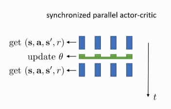
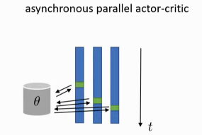
Online Actor-critic
 online actor-critic uses a single sample batch, which is a bad idea in
large neural networks. We need to use multiple samples to perform
updates.
online actor-critic uses a single sample batch, which is a bad idea in
large neural networks. We need to use multiple samples to perform
updates.
The purpose of multiple workers here is not to make the algorithm faster, but to make it work by increasing the batch size.
Generalized Advantage Estimation
\begin{equation} \hat{A}_{n}^\pi (s_t, a_t) = \sum_{t'=t}^{t+n}\gamma^{t’-t} r(s_{t’}, a_{t’}) - \hat{V}_{\phi}^\pi (s_t) + \gamma^n \hat{V}_\phi^\pi(s_{t+n}) \end{equation}
\begin{equation} \hat{A}_{GAE}^\pi (s_t, a_t) = \sum_{n=1}^{\infty} w_n \hat{A}_n^\pi (s_t, a_t) \end{equation}
is some weighted combination of n-step returns. If we choose \(w_n \propto \lambda^{n-1}\), we can show that:
\begin{equation} \hat{A}_{GAE}^\pi (s_t, a_t) = \sum_{n=1}^{\infty} (\gamma \lambda)^{t’-t} \delta_{t’} \end{equation}
where
\begin{equation} \delta_{t’} = r(s_{t’}, a_{t’}) + \gamma \hat{V}_\phi^\pi (s_{t'+1}) - \hat{V}_\phi^\pi(s_{t’}) \end{equation}
the role of \(\gamma\) and the role of \(\lambda\) turns out to b similar, trading off bias and variance!
Need to balance between learning speed, stability.
- Conservative Policy Iteration (CPI)
- propose surrogate objective, guarantee monotonic improvement under specific state distribution
- Trust Region Policy Optimization (TRPO)
- approximates CPI with trust region constraint
- Proximal Policy Optimization (PPO)
- replaces TRPO constraint with RL penalty + clipping (computationally efficient)
- Soft Actor-Critic (SAC)
- stabilize learning by jointly maximizing expected reward and policy entropy (based on maximum entropy RL)
- Optimistic Actor Critic (OAC)
- Focus on exploration in deep Actor critic approaches.
- Key insight: existing approaches tend to explore conservatively
- Key result: Optimistic exploration leads to efficient, stable learning in modern Actor Critic methods