Policy Gradients
Key Idea
The objective is:
\begin{equation} \theta^{\star}=\arg \max _{\theta} E_{\tau \sim p_{\theta}(\tau)}\left[\sum_{t} r\left(\mathbf{s}_{t}, \mathbf{a}_{t}\right)\right] \end{equation}
To evaluate the objective, we need to estimate this expectation, often through sampling by generating multiple samples from the distribution:
\begin{equation} J(\theta)=E_{\tau \sim p_{\theta}(\tau)}\left[\sum_{t} r\left(\mathbf{s}_{t}, \mathbf{a}_{t}\right)\right] \approx \frac{1}{N} \sum_{i} \sum_{t} r\left(\mathbf{s}_{i, t}, \mathbf{a}_{i, t}\right) \end{equation}
Recall that:
\begin{equation} \nabla_{\theta} J(\theta) \approx \frac{1}{N} \sum_{i=1}^{N} \underbrace{\nabla_{\theta} \log \pi_{\theta}\left(\tau_{i}\right)}_{\sum_{t=1}^{T} \nabla_{\theta} \log _{\theta} \pi_{\theta}\left(\mathbf{a}_{i, t} | \mathbf{s}_{i, t}\right)}r\left(\tau_{i}\right) \end{equation}
This makes the good stuff more likely, and bad stuff less likely, but scaled by the rewards.
Comparison to Maximum Likelihood
- policy gradient
- \(\nabla_{\theta} J(\theta) \approx \frac{1}{N} \sum_{i=1}^{N}\left(\sum_{t=1}^{T} \nabla_{\theta} \log \pi_{\theta}\left(\mathbf{a}_{i, t} | \mathbf{s}_{i, t}\right)\right)\left(\sum_{t=1}^{T} r\left(\mathbf{s}_{i, t}, \mathbf{a}_{i, t}\right)\right)\)
- maximum likelihood
- \(\nabla_{\theta} J_{\mathrm{ML}}(\theta) \approx \frac{1}{N} \sum_{i=1}^{N}\left(\sum_{t=1}^{T} \nabla_{\theta} \log \pi_{\theta}\left(\mathbf{a}_{i, t} | \mathbf{s}_{i, t}\right)\right)\)
Partial Observability
The policy gradient method does not assume that the system follows the Markovian Assumption! The algorithm only requires the ability to generate samples, and a function approximator for \(\pi_{\theta}(a_t |o_t)\).
Issues
- Policy gradients have high variance: the gradient is noisy, easily affected by a constant change in rewards
Properties of Policy gradients
- On-policy
The objective is an expectation under trajectories sampled under that policy. This can be tweaked into an off-policy method using Importance Sampling.
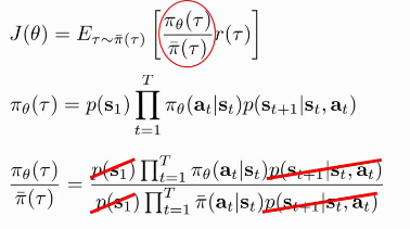
Figure 1: Off-policy policy gradients
\begin{align} \nabla_{\theta^{\prime}} J\left(\theta^{\prime}\right) &=E_{\tau \sim \pi_{\theta}(\tau)}\left[\frac{\pi_{\theta^{\prime}}(\tau)}{\pi_{\theta}(\tau)} \nabla_{\theta^{\prime}} \log \pi_{\theta^{\prime}}(\tau) r(\tau)\right] \quad \text { when } \theta \neq \theta^{\prime} \ &=E_{\tau \sim \pi_{\theta}(\tau)}\left[\left(\prod_{t=1}^{T} \frac{\pi_{\theta^{\prime}}\left(\mathbf{a}_{t} | \mathbf{s}_{t}\right)}{\pi_{\theta}\left(\mathbf{a}_{t} | \mathbf{s}_{t}\right)}\right)\left(\sum_{t=1}^{T} \nabla_{\theta^{\prime}} \log \pi_{\theta^{\prime}}\left(\mathbf{a}_{t} | \mathbf{s}_{t}\right)\right)\left(\sum_{t=1}^{T} r\left(\mathbf{s}_{t}, \mathbf{a}_{t}\right)\right)\right] \end{align}
Problem: with large T the first term becomes extremely big or small.
Variance Reduction
Causality
The policy at time \(t’\) cannot affect the reward at time \(t\) when \(t < t’\).
\begin{equation} \nabla_{\theta} J(\theta) \approx \frac{1}{N} \sum_{i=1}^{N}\left(\sum_{t=1}^{T} \nabla_{\theta} \log \pi_{\theta}\left(\mathbf{a}_{i, t} | \mathbf{s}_{i, t}\right)\right)\left(\sum_{t=t’}^{T} r\left(\mathbf{s}_{i, t}, \mathbf{a}_{i, t}\right)\right) \end{equation}
This is still an unbiased estimator, and has lower variance because the gradients are multiplied by smaller values. This is often written as:
\begin{equation} \nabla_{\theta} J(\theta) \approx \frac{1}{N} \sum_{i=1}^{N} \sum_{t=1}^{T} \nabla_{\theta} \log \pi_{\theta}\left(\mathbf{a}_{i, t} | \mathbf{s}_{i, t}\right) \hat{Q}_{i, t} \end{equation}
where \(\hat{Q}_{i,t}\) is the reward-to-go.
Baseline Reduction
\begin{equation} \nabla_{\theta} J(\theta) \approx \frac{1}{N} \sum_{i=1}^{N} \nabla_{\theta} \log \pi_{\theta}(\tau)[r(\tau)-b] \end{equation}
Subtracting a baseline is unbiased in expectation, but may reduce the variance. We can compute the optimal baseline, by evaluating the variance of the gradient, and setting the derivative of the variance with respect to \(b\) to 0:
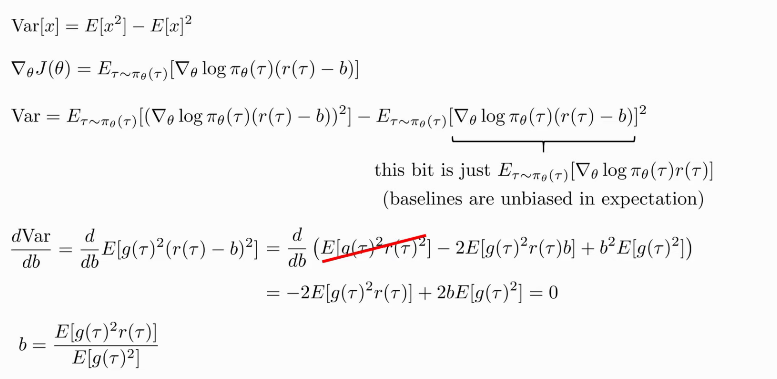
Figure 2: Computing the optimal baseline
This is just expected reward, but weighted by gradient magnitudes.
Policy Gradient in practice
- Gradients have high variance
- Consider using much larger batches
- Tweaking learning rates might be important
- Adaptive learning rates are fine, there are some policy-gradient oriented learning rate adjustment methods
REINFORCE
- For each episode,
- generate \(\tau = s_0, a_0, r_1, \dots, s_{t-1}, a_{t-1}, r_t\) by following \(\pi_{\theta}(a |s)\)
- For each step \(i = 0, \dots, t-1\):
- \(R_i = \sum_{k=i}^{t} \gamma^{t-k} r_k\) (Unbiased estimate of remaining episode return under \(\pi_{\theta}\) starting from \(i\))
- \(\hat{A_i} = R_i - b\) (Advantage function: subtract base line \(b\) to lower variance)
- Advantage function tells you how relatively good this action is
- $θ = \(\theta + \alpha \nabla_\theta \log \pi_{\theta} (a| s_i) \hat{A}_i\)
Objective: \(J(\theta) = \sum_{\tau} P_{\theta}(\tau)R(\tau)\)
\begin{align}
\nabla_\theta J(\theta) &= \nabla_\theta \sum_{\tau} P_\theta(\tau)
R(\tau) \\\
&= \sum_{\tau} \nabla_\theta P_\theta(\tau)R(\tau)
\end{align}
Actor critics use learned estimate (e.g. $\hat{A}(s, a) = \hat{Q}(s,
-
- \hat{V}(s).)
Policy Gradients an Policy Iteration
Policy gradients involves estimating \(\hat{A}{s,a}\), and using it to improve the policy, much like policy iteration which evaluates \(A(s,a)\) and use it to create a better, deterministic policy.
\begin{align}
J(\theta’) - J(\theta) &= J(\theta’) - E_{s_0 \sim p(s_1)}\left[
V^{\pi_\theta}(s_0) \right] \\\
&=J(\theta’) - E_{\tau \sim p_{\theta’}(\tau)}\left[
V^{\pi_\theta}(s_0) \right] \\\
&= J(\theta’) - E_{\tau \sim
p_{\theta’}(\tau)} \left[
\sum_{t=0}^{\infty} \gamma^t
V^{\pi_\theta} (s_t) - \sum_{t=1}^{\infty} \gamma^t
V^{\pi_\theta} (s_t)\right] \\\
&= J(\theta’) + E_{\tau \sim
p_{\theta’}(\tau)} \left[
\sum_{t=0}^{\infty} \gamma^t (\gamma
V^{\pi_\theta}(s_{t+1}) -
V^{\pi_\theta})(s_t) \right] \\\
&= E_{\tau \sim \p_{\theta’}(\tau)} \left[
\sum_{t=0}^{\infty} \gamma^t r(s_t, a_t)
\right] + E_{\tau \sim
p_{\theta’}(\tau)} \left[
\sum_{t=0}^{\infty} \gamma^t (\gamma
V^{\pi_\theta}(s_{t+1}) -
V^{\pi_\theta})(s_t) \right] \\\
&= E_{\tau \sim p_{\theta’}(\tau)} \left[
\sum_t \gamma^t A^{\pi_\theta} (s_t, a,_t) \right]
\end{align}
We have an expectation under \(\theta’\), but samples under \(\theta\). We use marginals representation, and Importance Sampling to remove the expectation under \(\pi_\theta’\), but can we ignore the other distribution mismatch?
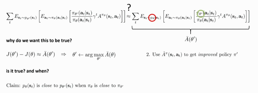
We can bound the distribution change from \(p_{\theta}(s_t)\) to \(p_{\theta’}(s_t)\). (See Trust Region Policy Optimization paper)
We can measure the distribution mismatch with KL divergence.
Then, we can enforce the constraint of a small KL divergence by using a loss function with the Lagrange Multiplier:
\begin{equation} L(\theta’, \lambda) = \sum_{t} E_{s_t \sim p_\theta(s_t)} \left[ E_{a_t \sim \pi_{theta}(a_t|s_t)} \left[ \frac{p_{theta’}(a_t|s_t)}{p_\theta(a_t|s_t)} \gamma^t A^{\pi_\theta} (s_t, a_t) \right] \right] - \lambda \left( D_{KL}(\pi_{\theta’}(a_t|s_t) || \pi_\theta (a_t|s_t)) - \epsilon \right) \end{equation}
- Maximize \(L’\) wrt to \(\theta’\)
- \(\lambda \leftarrow \lambda + \alpha (D_{KL} - \epsilon)\)
Intuition: raise \(\lambda\) if constraint violated too much, else lower it.
Alternatively, optimize within some region, and use a Taylor expansion to approximate the function within that region.