Q-Learning
The Actor-Critic algorithm fits 2 function approximators: one for the policy, and one for the value function. A key problem with the policy gradient method is the high variance in the gradient update. Can we omit Policy Gradients completely?
Key Ideas
- If we have a policy \(\pi\), and we know \(Q^{\pi}(s_t, a_t)\), then we can improve \(\pi\) by setting \(\pi’(a|s) = 1\) where \(a = \mathrm{argmax}_aQ^{\pi}(s , a)\).
- We can compute the gradient to increase the probability of good actions \(a\): if \(Q^{\pi}(s, a) > V^{\pi}(s)\), then a is better than average (\(V\) is expectation of \(Q\) over \(\pi(a|s)\)).
- It can be shown that in a fully-observed MDP, there is a policy that is both deterministic and optimal
Policy Iteration
- evaluate \(A^\pi (s, a)\)
- set \(\pi \leftarrow \pi’\) where \(\pi’ = 1\) if \(a_t = \mathrm{argmax}_{a_t}A^\pi(s_t, a_t)\) and \(0\) otherwise
Value Iteration
Skips the explicit policy representation altogether. Key idea: argmax of advantage function is the same as argmax of Q-function.
- set \(Q(s,a) \leftarrow r(s,a) + \gamma E\left[V(s’)\right]\)
- set \(V(s) \leftarrow \mathrm{argmax}_a Q(s,a)\)
This simplifies the dynamic programming problem in policy iteration.
Fitted Value Iteration
We can use any most function approximators to represent \(V(s)\).
- set \(y_i \leftarrow \mathrm{max}_{a_i} (r(s_i, a_i) + \gamma E\left[V_{\phi}(s_i’)\right])\)
- set \(\phi \leftarrow \mathrm{argmin}_{\phi} \frac{1}{2} \sum_i |V_{\phi}(s_i) - y_i |^2\)
This algorithm suffers from the curse of dimensionality. When the state space is large, the algorithm is computationally expensive. To get around this, we may sample states instead, with little change to the algorithm.
Fitted Q Iteration
Notice the \(\mathrm{max}\) over \(a_i\). This means that we need to know the outcomes for different actions! But what if we don’t know the transition dynamics? If we use a Q-table, then we arrive at an algorithm without needing to know the transition dynamics!
- set \(y_i \leftarrow r(s_i, a_i) + \gamma E\left[V_{\phi}(s_i’)\right]\)
- set \(\phi \leftarrow \mathrm{argmin}_{\phi} \frac{1}{2} \sum_i |Q_{\phi}(s_i, a_i) - y_i |^2\)
There is still a “max” hiding in \(V_\phi(s_i’)\). To get around this, we approximate \(E\left[V(s_i’)\right] \approx \mathrm{max}_{a’} Q(s_i’, a_i’)\):
- Collect dataset \(\left\{(s_i, a_i, s_i’, r_i)\right\}\) using some policy 1.1. set \(y_i \leftarrow r(s_i, a_i) + \gamma \mathrm{max}_{a’} Q(s_i’, a_i’)\) 1.2. set \(\phi \leftarrow \mathrm{argmin}_{\phi} \frac{1}{2} \sum_i |Q_{\phi}(s_i, a_i) - y_i |^2\) 1.3. goto 1.1 or 1
This works, even for off-policy samples (unlike Actor-Critic). In addition, there is only one network, hence no high-variance policy gradient methods. However, there are no convergence guarantees with non-linear function approximators!
Why is it off-policy? The algorithm doesn’t assume anything about the policy: given \(s\) and \(a\), the transition is independent of \(\pi\).
In step 1.3, if the algorithm is off-policy, why would we ever need to go back to collect more samples in step 1? This is because on a random, poorly performing policy, we might not access some interesting states, that we would get after learning a better policy through Q-iteration.
Exploration in Q-learning
The policy used in Q-learning is deterministic. To get around this, we use a different, stochastic policy in step 1, when sampling actions to take. An example of such a policy is the epsilon-greedy, or Boltzmann exploration policy.
Non-Tabular Value Function Learning
In the tabular case, we have a Bellman contraction \(BV\) such that \(B\) is a contraction w.r.t. tho infinity-norm:
\begin{equation} |BV - B\overline{V}| \le \gamma |V - \overline{V}| _{\infty} \end{equation}
When we do fitted value iteration, we have another contraction \(\Pi\) that is a contraction wr.t. the \(l_2\) norm (if we do the l2 norm regression):
\begin{equation} |\Pi V - \Pi\overline{V}| \le |V - \overline{V}| _{\infty} \end{equation}
However, \(\Pi B\) is not a contraction of any kind! All convergence guarantees is lost!
Q-learning is not gradient descent!
There are several problems with the regular Q-iteration algorithm:
- Samples are temporally correlated
- Target values are always changing
- There is a no gradient through the target value, even though it seems we are doing a single gradient update step.
- Single-sample updates
With 1 and 2, it’s possible to repeatedly overfit to the current sample.
Dealing with correlated samples
We can follow the same technique from actor-critic (synchronous/asynchronous parallel Q-learning) to alleviate correlated samples. The samples are however still temporally correlated. A better solution is to use a replay buffer.
Replay buffer
We have a buffer \(B\) that stores samples of \((s_i, a_i, s_i’, r_i)\) Each time we do an update, we sample a batch i.i.d from \(B\), resulting in a lower-variance gradient. The i.i.d results in decorrelated samples. In practice, we periodically update the replay buffer.
Dealing with the moving target
In the online Q-learning algorithm, the target Q moves. To resolve this we can use a target network:
\begin{equation} \phi \leftarrow \phi - \alpha \sum_i \frac{dQ_\phi}{d\phi}(s_i,a_i)(Q_\phi(s_i,a_i) - [r(s_i,a_i) + \gamma Q_{\phi ‘}(s_i’, a_i’)]) \end{equation}
The use of the target network \(Q_{\phi ‘}\) results in targets not changing in the inner loop.
DQN
DQN is the result of using a replay buffer, target network and some gradient clipping. See Playing Atari with Deep RL.
Double DQN
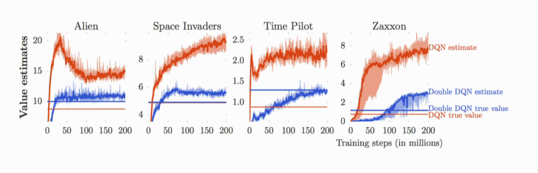
Figure 1: The predicted Q-values are much higher than the true Q-values
It has been shown imperatively that the learnt Q-values are numerically much higher than the true Q-values. Practically, this isn’t much of an issue: as the predicted Q-value increases, performance also increases.
The intuition behind why this happens, is that our target value \(y_j\) is given by:
\begin{equation} y_j = r_j + \gamma \mathrm{max}_{a_j’}Q_{\phi ‘}(s_j’, a_j’) \end{equation}
It is easy to show that:
\begin{equation} E\left[ \mathrm{max}(X_1, X_2) \right] \ge \mathrm{max}(E[X_1], E[X_2]) \end{equation}
\(Q_{\phi ‘}(s’, a’)\) overestimates the next value, because it is noisy! The solution is to use 2 Q-functions, decorrelating the errors:
\begin{equation} \mathrm{max}_{a’}Q_{\phi ‘}(s’, a’) = Q_{\phi ‘}(s’, \mathrm{argmax}_{a’}(s’,a’)) \end{equation}
becomes:
\begin{equation} Q_{\phi_A} (s,a) \leftarrow r + \gamma Q_{\phi_B}(s’, \mathrm{argmax}_{a’}Q_{\phi_A}(s’,a’)) \end{equation}
\begin{equation} Q_{\phi_B} (s,a) \leftarrow r + \gamma Q_{\phi_A}(s’, \mathrm{argmax}_{a’}Q_{\phi_B}(s’,a’)) \end{equation}
To get 2 Q-functions, we use the current and target networks:
\begin{equation} y = r + \gamma Q_{\phi ‘}(s’, \mathrm{argmax}_{a’} Q_\phi(s’,a’)) \end{equation}
Q-learning with stochastic optimization
Taking max over a continuous action space can be expensive. A simple approximation is:
\begin{equation} \mathrm{max}_{a} Q(s,a) \approx \mathrm{max}\left\{ Q(s,a_1), \dots, Q(s,a_N)\right\} \end{equation}
where \((a_1, \dots, a_N)\) is sampled from some distribution. A more accurate solution is to use the cross-entropy method.
Another option is to use a function class that is easy to maximize (e.g. using a quadratic function). This option is simple, but loses representational power.
The final option is to learn an approximate maximizer (e.g. DDPG). The idea is to train another network \(\mu_{\phi}(s) \approx \mathrm{argmax}_{a}Q_{\phi}(s,a)\), by solving \(\theta \leftarrow \mathrm{argmax} Q_\phi(s, \mu_\theta(s))\)
Q-learning
Q-learning learns an action-utility representation instead of learning utilities. We will use the notation \(Q(s,a)\) to denote the value of doing action \(a\) in state \(s\).
\begin{equation} U = max_a Q(s, a) \end{equation}
A TD agent that learns a Q-function does not need a model of the form \(P(s’ | s, a)\), either for learning or for action selection. Q-learning is hence called a model-free method. We can write a constraint equation as follows:
\begin{equation} Q(s,a) = R(s) + \gamma \sum_{s’} P(s’ | s, a) max_{a’} Q(s’, a’) \end{equation}
However, this equation requires a model to be learnt, since it depends on \(P(s’ | s, a)\). The TD approach requires no model of state transitions.
The updated equation for TD Q-learning is:
\begin{equation} Q(s, a) \leftarrow Q(s, a) + \alpha (R(s) + \gamma max_{a’} Q(s’, a’) - Q(s,a)) \end{equation}
which is calculated whenever action \(a\) is executed in state \(s\) leading to state \(s’\).
Q-learning has a close relative called SARSA (State-Action-Reward-State-Action). The update rule for SARSA is as follows:
\begin{equation} Q(s, a) \leftarrow Q(s, a) + \alpha (R(s) + \gamma Q(s’, a’) - Q(s, a)) \end{equation}
where \(a’\) is the action actually taken in state \(s’\). The rule is applied at the end of each \(s, a, r, s’, a’\) quintuplet, hence the name.
Whereas Q-learning backs up the best Q-value from the state reached in the observed transition, SARSA waits until an action is actually taken and backs up the Q-value for that action. For a greedy agent that always takes the action with best Q-value, the two algorithms are identical. When exploration is happening, they differ significanty.
Because Q-learning uses the best Q-value, it pays no attention to the actual policy being followed - it is an off-policy learning algorithm. However, SARSA is an on-policy algorithm.
Q-learning is more flexible in the sense that a Q-learning agent can learn how to behave well even when guided by a random or adversarial exploration policy. On the other hand, SARSA is more realistic: for example if the overall policy is even partly controlled by other agents, it is better to learn a Q-function for what will actually happen rather than what the agent would like to happen.
Q-learning has been shown to be sample efficient in the tabular setting (Jin et al., n.d.).
Q-learning with function approximation
To generalize over states and actions, parameterize Q with a function approximator, e.g. a neural net:
\begin{equation} \delta = r_t + \gamma \mathrm{max}_a Q(s_{t+1}, a; \theta) - Q(s_t, a ; \theta) \end{equation}
and turn this into an optimization problem minimizing the loss on the TD error:
\begin{equation} J(\theta) = \left| \delta \right|^2 \end{equation}
The key problem with Q-learning is stability, coined the “deadly triad”.
- Off-policy learning
- flexible function approximation
- Bootstrapping
In the presence of all three, learning is unstable. DQN is the first algorithm that stabilized deep Q-learning (Playing Atari with Deep RL).
Bibliography
Jin, Chi, Zeyuan Allen-Zhu, Sebastien Bubeck, and Michael I Jordan. n.d. “Is Q-Learning Provably Efficient?” In Advances in Neural Information Processing Systems 31, edited by S. Bengio, H. Wallach, H. Larochelle, K. Grauman, N. Cesa-Bianchi, and R. Garnett, 4863–73. Curran Associates, Inc. http://papers.nips.cc/paper/7735-is-q-learning-provably-efficient.pdf.