Natural Language Processing
How to Represent Words
http://ruder.io/word-embeddings-2017/index.html
How do we represent words as input to any of our models? There are an estimated 13 million tokens for the English language, some of them have similar meanings.
The simplest representation is one-hot vector: we can represent every word as a \(\mathbb{R}^{|V|x}\) vector with all 0s and one 1 at the index of that word in the sorted english language.
To reduce the size of this space, we can use SVD-based methods. For
instance, accumulating co-occurrence count into a matrix X, and
perform SVD on X to get a \(USV^T\) decomposition. We can then use the
rows of U as the word embeddings for all words in the dictionary.
Window-based Co-occurence Matrix
Count the number of times each word appears inside a window of a particular size around the word of interest. We calculate this count for all words in the corpus.
Issues with SVD-based methods
- Dimensions of the matrix can change very often (new words added to corpus)
- Matrix is extremely sparse as most words don’t co-occur
- Matrix is very high-dimensional
- Quadratic cost to perform SVD
Some solutions include:
- Ignore function words (blacklist)
- Apply a ramp window (distance between words)
- Use Pearson correlation and set negative counts to 0 instead of raw count.
Iteration-based Methods (e.g. word2vec)
Design a model whose parameters are the word vectors, and train the model on a certain objective. Discard the model, and use the vectors learnt.
Efficient tree structure to compute probabiltiies for all the vocabulary
Language Models
The model will need to assign a probability to a sequence of tokens. We want a high probability for a sentence that makes sense, and a low probability for a sentence that doesn’t.
Unigrams completely ignore this, and a nonsensical sentence might actually be assigned a high probability. Bigrams are a naive way of evaluating a whole sentence.
-
Continuous bag-of-words (CBOW)
Predicts a center word from the surrounding context in terms of word vectors.
For each word, we want to learn 2 vectors:
-
v: (input vector) when the word is in the context
-
u: (output vector) when the word is in the center
-
known parameters
- input: sentence represented by one-hot vectors
- output: one hot vector of the known center word
Create 2 matrices \(\mathbb{V} \in \mathbb{R}^{n \times |V|}\) and \(\mathbb{U} \in \mathbb{R}^{|V| \times n}\), where n is the arbitrary size which defines the size of the embedding space.
\(V\) is the input word matrix such that the i-th column of \(V\) is the $n$-dimensional embedded vector for word \(w_i\) when it is an input to this model. \(U\) is the output word matrix.
- Generate one-hot word vectors for the input context of size m.
- Get our embedded word vectors for the context: (\(v_{c-m} = Vx^{c-m}\), …)
- Average these vectors to get \(\hat{v} = \frac{\sum v}{2m} \in \mathbb{R^n}\)
- Generate a score vector \(z = U\hat{v} \in \mathbb{R}^{|V|}\) As the dot product of similar vectors is higher, it will push simila words close to each other in order to achieve a high score.
- Turn the scores into probabilities \(\hat{y} = softmax(z) \in \mathbb{R}^{|V|}\)
Minimise loss function (cross entropy), and use stochastic gradient descent to update all relevant word vectors.
-
-
Skipgram
http://mccormickml.com/2016/04/19/word2vec-tutorial-the-skip-gram-model/
Predicts the distribution of context words from a center word. This is very similar to the CBOW approach, wind the input and output vectors reversed. Here, a naive Bayes assumption is invoked: that given the center word, all output words are completely independent.
Input vector: one-hot vectors corresponding to the vocabulary
The neural network is consists of one hidden layer of \(n\) units, where \(n\) is the desired dimension of the word vector. The output layer is a softmax regression layer, outputting a value between 0 and 1. We want the value for the context words to be high, and the non-context words to be low.
After training, the output layer is discarded, and the weights at the hidden layer are the word vectors we want.
Training Methods
In practice, negative sampling works better for frequently occurring words and lower-dimensional vectors, and hierachical softmax works better for infrequent words.
-
Negative Sampling
Take \(k\) negative samples, and minimise the probability of the two words co-occurring while also maximising the probability of the two words in the same window co-occur.
-
Hierarchical Softmax
Hierarchical Softmax uses a binary tree to represent all words in the vocabulary. Each leaf of the tree is a word, and there is a unique path from root to leaf. The probability of a word \(w\) given a vector \(w_i\), \(P(w|w_i)\), is equal to the probability of a random walk starting from the root and ending in the leaf node corresponding to \(w\).
Global Vectors for Word Representation (GloVe)
Count-based methods of generating word embeddings rely on global statistical information, and do poorly on tasks such as word analogy, indicating a sub-optimal vector space structure.
word2vec presents a window-based method of generating word-embeddings by making predictions in context-based windows, demonstrating the capacity to capture complex linguistic patterns beyond word similarity.
GloVe consists of a weighted least-squares model that combines the benefits of the word2vec skip-gram model when it comes to word analogy tasks, but also trains on global word-word co-occurrence counts, and produces a word vector space with meaningful sub-structure.
The appropriate starting point for word-vector learning should be with ratios of co-occurrence probabilities rather than the probabilities themselves. Since vector spaces are inherently linear structures, the most natural way to encode the information present in a ratio in the word vector space is with vector differences.
The training objective of GloVe is to learn word vectors such that their dot product equals the logarithm of the words’ probability of co-occurrence. Owing to the fact that the logarithm of a ratio equals the difference of logarithms, this objective associates (the logarithm of) ratios of co-occurrence probabilities with vector differences in the word vector space.
Co-occurrence Matrix
Let \(X\) denote the word-word co-occurrence matrix, where \(X_{ij}\) indicate the number of times word \(j\) occur in the context of word \(i\). Let \(X_i = \sum_k X_{ik}\) be the number of times any word \(k\) appears in the context of word \(i\). Let \(P_{ij} = P(w_j|w_i) = \frac{X_{ij}}{X_i}\) be the probability of j appearing in the context of word \(i\).
Topic Modeling
- Topics are distributions over keywords
- Documents are distributions over topics
Topic summaries are NOT perfect. UTOPIAN allows user interactions for improving them.
Topic Lens https://ieeexplore.ieee.org/document/7539597/ UTOPIAN http://xueshu.baidu.com/s?wd=paperuri%3A%2809451ca1aa2a439f5b6e0c6c768fcd9a%29&filter=sc%5Flong%5Fsign&tn=SE%5Fxueshusource%5F2kduw22v&sc%5Fvurl=http%3A%2F%2Fieeexplore.ieee.org%2Fdocument%2F6634167%2F&ie=utf-8&sc%5Fus=618112135367870968
Dimension Reduction
Multidimensional Scaling
- Tries to preserve given pairwise distances in a low-dimensional space.
Word Vector Evaluation
Intrinsic
- Evaluation on a specific/intermediate subtask
- Fast to compute
- Helps understand the system
- Not clear if really helpful unless correlation to real task is established
Extrinsic
- Evaluation on a real task
- Can take a long time to compute accuracy
- Unclear if the subsystem is the problem or its interaction or other subsystems
- If replacing exactly one subsystem with another improves accuracy ➡ Winning!
Visualizing Word Embeddings
Neural Networks
Most data are not linearly separable, hence the need for non-linear classifiers. Neural networks are a family of classifiers with non-linear decision boundaries.
A neuron
A neuron is a generic computational unit that takes \(n\) inputs and produces a single output. The sigmoid unit takes a $n$-dimensional vector $x4 and produces a scalar activation (output) \(a\). This neuron is also associated with an $n$-dimensional weight vector, \(w\), and a bias scalar, \(b\). for example, the output of this neuron is then:
\begin{equation*} a = \frac{1}{1 + exp(-(w^Tx + b))} \end{equation*}
This is also frequently formulated as:
\begin{equation*} a = \frac{1}{1 + exp(-([w^T\text{ }b] \cdot [x\text{ }1]))} \end{equation*}
A single layer of neurons
This idea can be extended to multiple neurons by considering the case where the input \(x\) is fed as input to multiple such neurons.
\begin{align*}
\sigma\left( z \right) =
\begin{bmatrix}
\frac{1}{1 + exp(z_1)} \\\
\vdots \\\
\frac{1}{1 + exp(z_m)}
\end{bmatrix}
\end{align*}
\begin{align*}
b =
\begin{bmatrix}
b_1 \\\
\vdots \\\
b_m
\end{bmatrix}
\in \mathbb{R}^m
\end{align*}
\begin{align*}
W =
\begin{bmatrix}
- && w^{(1)T} && - \\\
&& \dots && \\\
- && w^{(m)T} && -
\end{bmatrix}
\in \mathbb{R}^{m\times n}
\end{align*}
\begin{equation*} z = Wx + b \end{equation*}
The activations of the sigmoid function can be written as:
\begin{align*}
\begin{bmatrix}
a^{(1)} \\\
\vdots \\\
a^{(m)}
\end{bmatrix}
= \sigma\left( Wx + b \right)
\end{align*}
Activations indicate the presence of some weighted combination of features. We can use these combinations to perform classification tasks.
Feed-forward computation
Non-linear decisions cannot be classified in by feeding inputs directly into a softmax function. Instead, we use another matrix \(U \in \mathbb{R}^{m\times 1}\) to generate an unnormalized score for a classification task from the activations.
\begin{equation*} s = U^Ta = U^Tf\left( Wx + b \right) \end{equation*}
where f is the activation function.
Maximum Margin Objective Function
Neural networks also need an optimisation objective. the maximum margin objective ensures that the score computed for “true” labeled data points is higher than the score computed for “false” labeled data points, i.e. \(\text{minimize} J = max(s_c - s, 0)\), where \(s_c\) is the corrupt false window. This optimization can be achieved through backpropagation and gradient descent.
Gradient Checks
One can numerically approximate these gradients, allowing us to precisely estimate the derivative with respect to any parameter, serving as a sanity check on the correctness of our analytic derivatives.
\begin{equation*} f’(\theta) = \frac{J(\theta^{i+}) - J(\theta^{i-})}{2\epsilon} \end{equation*}
Dependency Parsing
Dependency Grammar and Dependency Structure
Parse trees in NLP are used to analyse the syntatic structure of sentences.
Consistency Grammar uses phrase structure grammar to organize words into nested constituents.
Dependency structure of sentences shows which words depend on (modify or are arguments of) other words. These binary assymetric relations between words are called dependencies and are depicted as arrows going from the head to the dependent. Usually these dependencies form a tree structure.
Dependency Parsing
Dependency parsing is the task of analysing the syntactic dependency structure of a given input sentence S. The output of a dependency parser is a dependency tree where the words of the input sentence are connected by typed dependency relations.
Formally, the dependency parsing problem asks to create a mapping from the input sentence with words \(S = w_0w_1\dots w_n\) (where \(w_0\) is the ROOT) to its dependency graph \(G\).
The two subproblems are:
- Learning
- Given a training set \(D\) of sentences annotated with dependency graphs, induce a parsing model \(M\) that can be used to parse new sentences.
- Parsing
- Given a parsing model \(M\), and a sentence \(S\), derive the optimal dependency graph \(D\) for \(S\) according to \(M\).
Transition-based Parsing
This relies on a state machine which defines the possible transitions to create the mapping from the input sentence to the dependency tree. The learning problem involves predicting the next transition in the state machine. The parsing problem constructs the optimal sequence of transitions for the input sentence, given the previously induced model.
Greedy Deterministic Transition-based Parsing
The transition system is a state machine, which consists of states and transitions between those states. The model induces a sequence of transitions from some initial state to one of several terminal states. For any sentence \(S = w_0w_1\dots w_n\) a state can be described with a triple \(c = \left(\sigma, \beta, A)\):
- a stack \(\sigma\) of words \(w_i\) from S,
- a buffer \(\beta\) of words \(w_i\) from S,
- a set of dependency arcs \(A\) of the form \(\left(w_i, r, w_j\right)\)
For each sentence, there is an initial state, and a terminal state.
There are three types of transitions:
- shift
- Remove the first word in the buffer, and push it on top of the stack
- left-arc
- add a dependency arc \((w_j, r, w_i)\) to the arc set A, where \(w_i\) is the word second to the top of the stack, and \(w_j\) is the word at the top of the stack. Remove \(w_i\) from the stack.
- right-arc
- add a dependency arc \((w_i, r, w_j)\) to the arc set A, where \(w_i\) is the word second to the top of the stack, and \(w_j\) is the word at the top of the stack. Remove \(w_i\) from the stack.
Neural Dependency Parsing
-
Feature Selection
\(S_{word}\) : vector representation of the words in 4s$
\(S_{tag}\) : Part-of-Speech (POS) tags, comprising of a small discrete set \(P = {NN, NP, \dots}\)
\(S_{label}\) : Arc-labels, comprising of a small discrete set, describing the dependency relation.
For each feature type, we will have a corresponding embedding matrix, mapping from the feature’s one-hot encoding, to a d-dimensional dense vector representation.
The full embedding for \(S_{word}\) is \(E^w \in \mathbb{R}^{d\times N_w}\) where \(N_w\) is the vocabulary size. The POS and label embedding matrices are \(E^t \in \mathbb{R}^{d\times N_t}\) and \(E^l \in \mathbb{R}^{d\times N_l}\) where \(N_t\) and \(N_l\) are the number of distinct POS tags and arc labels respectively.
-
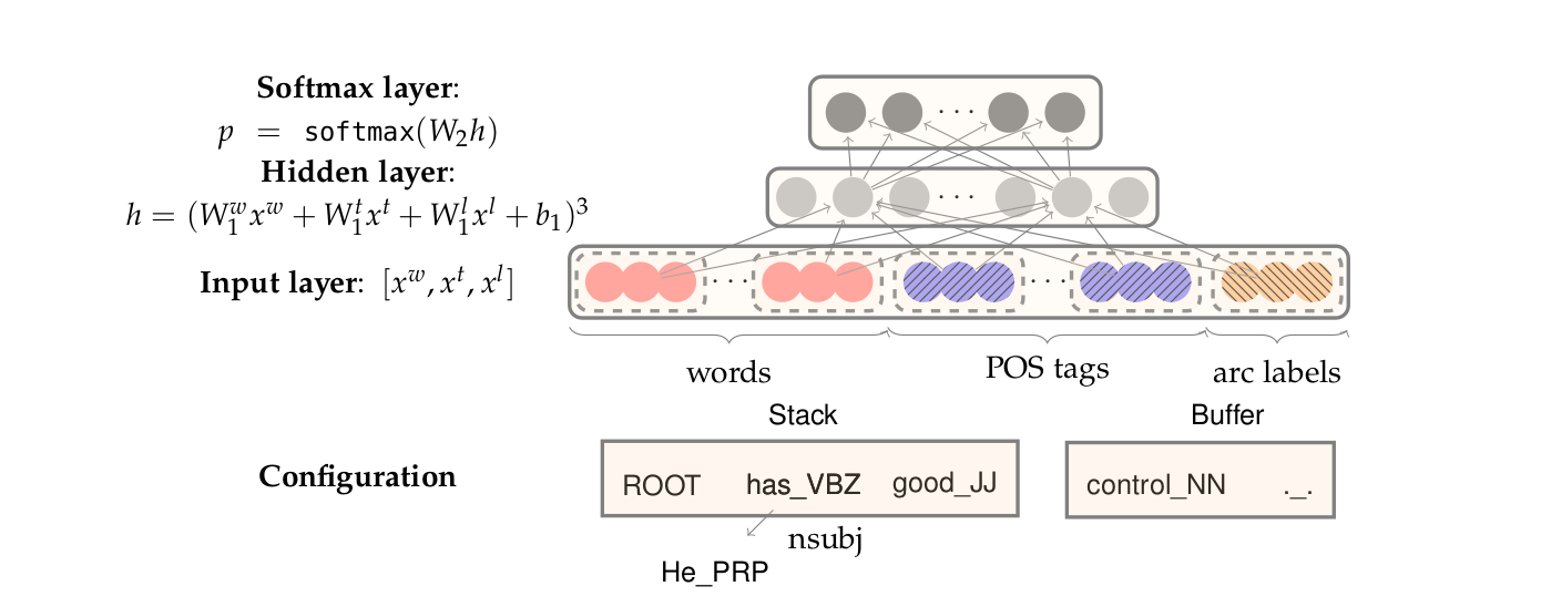
The network
The network contains an input layer \([x^w, x^t, x_l]\), a hidden layer, and a final softmax layer with a cross-entropy loss function.
We can define a single weight matrix in the hidden layer, to operate on a concatenation of \([x^w, x^t, x^l]\), or we can use three weight matrices \([W^w_1, W^t_1, W^l_1]\), one for each input type. We then apply a non-linear function and use one more affine (fully-connected) layer \([W_2]\) so that there are an equivalent number of softmax probabilities to the number of possible transitions (the output dimension).
Basic Visualization Techniques of Text Data
Word Cloud
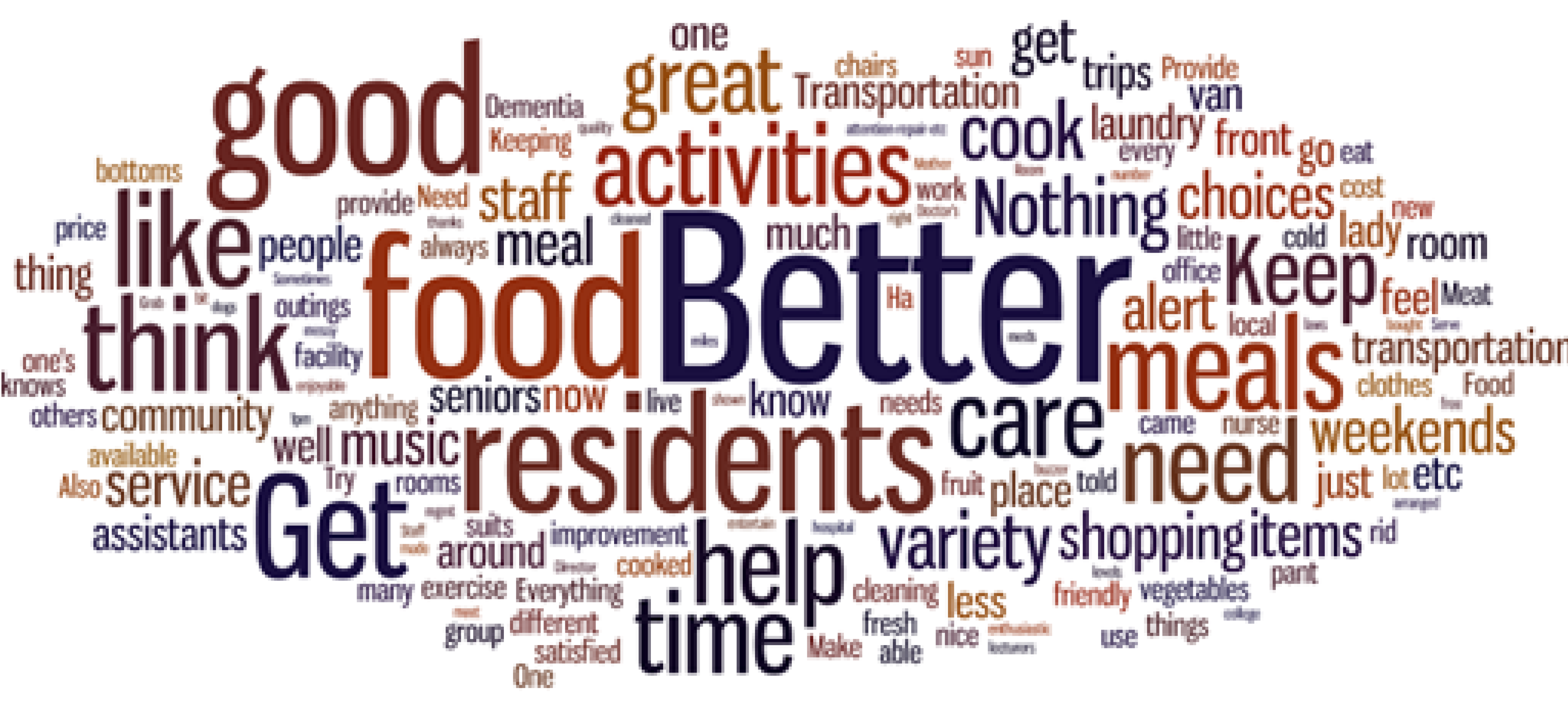
In word cloud, it is difficult to determine optimal placing of words. In addition, word clouds do not show relation between words.
Word Tree
ThemeRiver
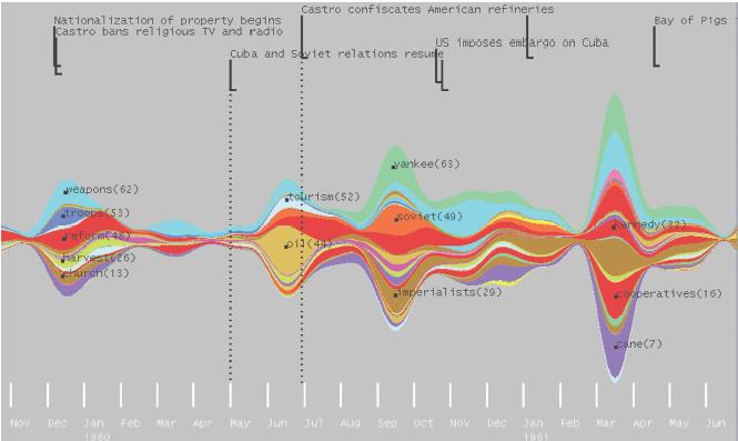
Time-series representation: view which keywords occur more frequently over time. It is a type of visualization known as a stacked linegraph.
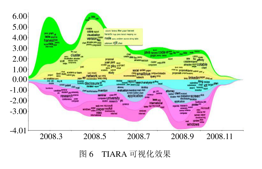
TIARA Visualization
Phrase Nets
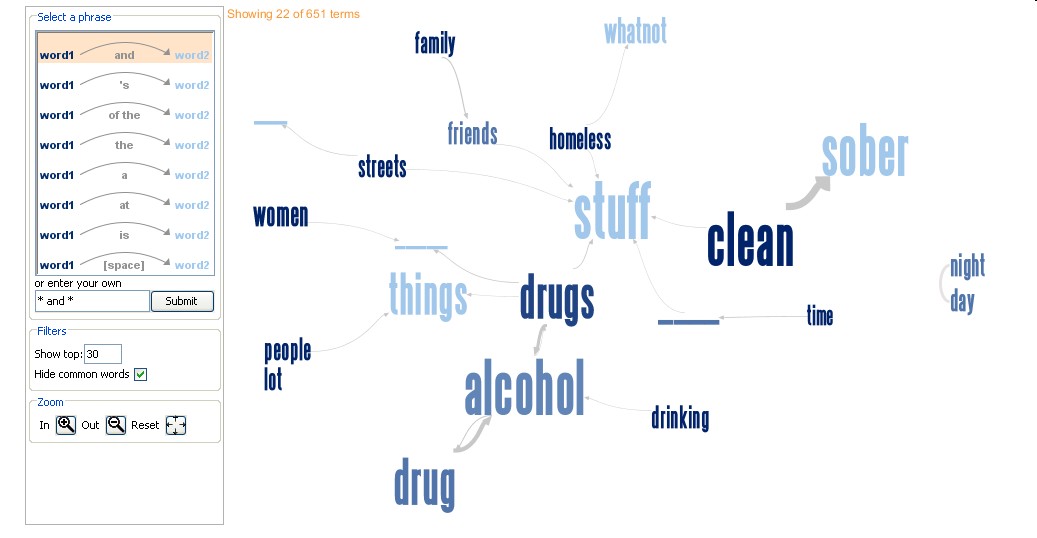
Phrasenets are useful for exploring how words are linked in a text and like word clouds and word trees can be informative for early data analysis.
For more…
http://textvis.lnu.se/ http://www.shixialiu.com