Machine Learning
When do we need machine learning?
Two aspects of a given problem may call for the use of programs that learn and improve on the basis of their “experience”:
-
The problem’s complexity: some tasks that require elaborate introspection that cannot be well-defined in programs, such as driving, are ill-suited for coding by hand. Tasks that are beyond human capabilities such as the analysis of large datasets also fall in this category.
-
Adaptivity: Programmed tools are rigid, while machine learning tools allows for adaptation to the environment they interact with.
Training vs Testing
Growth Function
The growth function is the quantity that will formalize the effective number of hypotheses.
Each \(h \in H\) generates a dichotomy which is \(h\) is \(-1\) or \(h\) i- \(+1\). We then formally define dichotomies as follows:
\begin{align} H(x_1, \dots, x_n) = \left\{ h(x_1), h(x_2), \dots, h(x_n) | h \in H \right\} \end{align}
Decision Tree Learning
Decision Tree Learning is a method of learning which approximates discrete-valued functions that is robust to noisy data, and is capable of learning disjunctive expressions
It is most appropriate when:
- instances are represented as attribute pairs
- the target function has discrete output values
- Disjunctive descriptions may be required
- The training data may contain errors
- The training data may contain missing attribute values
ID3 algorithm
ID3 learns decision trees by constructing them top down. Each instance attribute is evaluated using a statistical test to determine how well it alone classifies the examples. The best attribute is selected and used as the test at the root node of the tree.
Which is the best attribute?
A statistical property called information gain measures how well a given attribute separates the training examples according to their target classification.
Information gain is the expected reduction in entropy caused by partitioning the examples according to this attribute:
\begin{align} Gain(S,A) = Entropy(S) - \sum_{v\in Values(A)}\frac{|S_v|}{|S|}Entropy(S_v) \end{align}
For example:
\begin{align}
Values(Wind) &= Weak, Strong \\\
S &= [9+, 5-] \\\
S_{Weak} &\leftarrow [6+, 2-] \\\
S_{Strong} &\leftarrow [3+, 3-] \\\
Gain(S, Wind) &= Entropy(S) - \frac{8}{14}Entropy(S_{Weak}) -
\frac{6}{14}Entropy(S_{Strong}) \\\
&=0.048
\end{align}
Hypothesis Space Search
ID3 can be characterised as searching a space of hypotheses for one that fits the training examples. The hypothesis space searched is the set of possible decision trees. ID3 performs a simple-to-complex, hill-climbing search. The evaluation measure that guides the search is the information gain measure.
Because ID3’s hypothesis space of all decision trees is a complete space of finite discrete-valued functions, it avoids the risk that the hypothesis space might not contain the target function.
ID3 maintains only a single hypothesis as it searches through the space of decision trees. ID3 loses the capabilities that follow from explicitly representing all consistent hypothesis.
ID3 in its pure form performs no backtracking in its search, and can result in locally but not globally optimal target functions.
ID3 uses all training examples at each step to make statistically based decisions, unlike other algorithms that make decisions incrementally.
Inductive bias
The inductive bias of decision tree learning is that shorter trees are preferred over larger trees (Occam’s razor). Trees that place high information gain attributes close to the root are preferred over those that do not. ID3 can be viewed as a greedy heuristic search for the shortest tree without conducting the entire breadth-first search through the hypothesis space.
Notice that ID3 searches a complete hypothesis space incompletely, and candidate-elimination searches an incomplete hypothesis space completely. The inductive bias of ID3 follows from its search strategy (preference bias), while that of candidate elimination follows from the definition of its search space. (restriction bias).
Why Prefer Shorter Hypotheses?
- fewer shorter hypothesis than larger ones, means it’s less likely to over-generalise
Density Estimation
Density Estimation refers to the problem of modeling the probability distribution \(p(x)\) of a random variable \(x\), given a finite set \(x_1, x_2, \dots, x_n\) of observations.
We first look at parametric distributions, which are governed by a small number of adaptive parameters. In a frequentist treatment, we choose specific values for the parameters optimizing some criterion, such as the likelihood function. In a Bayesian treatment, we introduce prior distributions and then use Bayes’ theorem to compute the corresponding posterior distribution given the observed data.
An important role is played by conjugate priors, which yield posterior distributions of the same functional form.
The maximum likelihood setting for parameters can give severely over-fitted results for small data sets. To develop a Bayesian treatment to this problem, we consider a form of prior distribution with similar form as the maximum likelihood function. this property is called conjugacy. For a binomial distribution, we can choose the beta distribution as the prior.
Unsupervised Learning
In unsupervised learning, given a training set \(S = \left(x_1, \dots, x_m\right)\), without a labeled output, one must construct a “good” model/description of the data.
Example use cases include:
- clustering
- dimension reduction to ind essential parts of the data and reduce noise (e.g. PCA)
- minimises description length of data
K-means Clustering
Input: \(\{x^{(1), x^{(2)}, x^{(3)}, \dots, x^{(m)}}\}\).
- Randomly initialize cluster centroids.
- For all points, compute which cluster centroid is the closest.
- For each cluster centroid, move centroids to the average points belonging to the cluster.
- Repeat until convergence.
K-means is guaranteed to converge. To show this, we define a distortion function:
\begin{equation} J(c, \mu) = \sum_{i=1}^m || x^{(i)} - \mu_{c^{(i)}}||^2 \end{equation}
K means is coordinate ascent on J. Since \(J\) always decreases, the algorithm converges.
Gaussian Mixture Model
By Bayes’ Theorem:
\begin{equation} P(X^{(i)}, Z^{(i)}) = P(X^{(i)} | Z^{(i)})P(Z^{(i)}) \end{equation}
\begin{equation} Z^{(i)} \sim \text{multinomial}(\phi) \end{equation}
\begin{equation} X^{(i)} | Z^{(j)} \sim \mathcal{N}(\mu_j, \Sigma_j) \end{equation}
Refile
Data Compression
In lossy compression, we seek to trade off code length with reconstruction error.
In vector quantization, we seek a small set of vectors \({z_i}\) to describe a large dataset of vectors \({x_i}\), such that we can represent each \(x-i\) with its closest approximation in \({z_i}\) with small error. (Clustering problem)
In transform coding, we transform the data, usually using a linear tranformation. The data in the transformed domain is quantized, usually discarding the small coefficients, corresponding to removing some of the dimensions.
Generative Learning Algorithms
Discriminative algorithms model \(p(y | x)\) directly from the training set.
Generative algorithms model \(p(y | x)\) and \(p(y)\). Then \(argmax_y p(y|x) = argmax_y \frac{p(x|y)p(y)}{p(x)} = argmax_y p(x|y)p(y)\).
Multivariate Normal Distribution
A multivariate normal distribution is parameterized by a mean vector \(\mu \in R^n\) and a covariance matrix \(\Sigma \in R^{n \times n}\), where \(\Sigma \ge 0\) is symmetric and positive semi-definite.
TODO Gaussian Discriminant Analysis
In Gaussian Discriminant Analysis, p(x | y) is distributed to a Multivariate Normal Distribution.
\begin{align}
y &\sim Bernoulli(\phi) \\\
x|y = 0 &\sim N(\mu_0, \Sigma) \\\
x|y = 1 &\sim N(\mu_1, \Sigma)
\end{align}
We can write out the distributions:
\begin{align}
p(y) &= \phi^y (1 - \phi)^{1-y} \\\
p(x | y = 0) &= \frac{1}{(2\pi)^{n/2}|\Sigma|^{n/2}} exp \left( - \frac{1}{2} (x - \mu_0)^T \Sigma^{-1}(x - \mu_0) \right) \\\
p(x | y = 1) &= \frac{1}{(2\pi)^{n/2}|\Sigma|^{n/2}} exp \left( - \frac{1}{2} (x - \mu_1)^T \Sigma^{-1}(x - \mu_1) \right)
\end{align}
Then, the log-likelihood of the data is:
\begin{align}
l(\phi, \mu_0, \mu_1, \Sigma) &= \log \prod_{i=1}^m p(x^{(i)}, y^{(i)}; \mu_0, \mu_1, \Sigma) \\\
&= \log \prod_{i=1}^m p(x^{(i) }| y^{(i)}; \mu_0, \mu_1, \Sigma)p(y^{(i)}; \phi)
\end{align}
We maximize \(l\) with respect to the parameters.
The Natural Language Decathlon: Multitask Learning as Question Answering: Richard Socher
- Joint work with Bryan McCann, Nitish Keskar and Caiming Xiong
Limits of Single-task Learning
- We can hill climb to local optima if \(|dataset| > 100 \times C\)
- For more general model, we need continuous learning in a single model
For pre-training in NLP, we’re still stuck at the word vector level. This compared to vision, where most of the model can be pre-trained, only retraining the final few layers.
Why has weight & model sharing not happened so much in NLP?
- NLP requires many types of reasoning: logical, linguistic etc.
- Requires short and long-term memory
- NLP has been divided into intermediate and separate tasks to make progress (Benchmark chasing in each community)
- Can a single unsupervised task solve it all? No, language clearly requires supervision in nature.
Motivation for Single Multitask model
- Step towards AGI
- Important building block for:
- Sharing weights
- Transfer learning
- Zero-shot learning
- Domain adaptation
- Easier deployment in production
- Lowering the bar for anybody to solve their NLP task
End2end model vs parsing as intermediate step (e.g. running POS tagger first).
The 3 equivalent supertasks of NLP
Any NLP task can be mapped to these 3 super tasks:
- Language Modeling
- Question Answering
- Dialogue
Multitask learning as QA
- Question Answering
- Machine Translation
- Summarization
- NLI
- Sentiment Classification
- Semantic Role Labeling
- Relation Extraction
Meta supervised learning: {x, y} to {x, t, y}
Designing a model for decaNLP
- No task-specific modules or parameters because task ID assumed to be unavailable
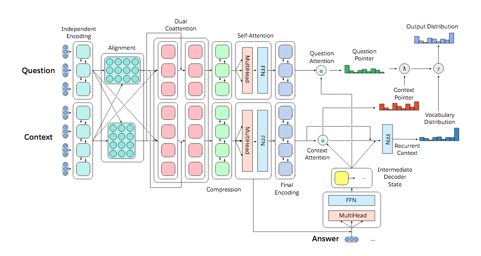
- Start with a context
- Ask a question
- Generate answer one at a time by
- Pointing to context
- Pointing to question
- Choosing a word
Learnings
- Transformer Layers yield benefits in single-task and multitask setting
- QA and SRL have strong connections
- Pointing to the question is essential, despite the task being just classification for some subtasks
- Mulitasking helps a lot with zero-shot tasks
(Latest version of the paper coming out soon – ICLR 2018)
Training Strategies
- Fully Joint
- Curriculum learning doesn’t work
- Anti-curriculum training works instead
- Start with a really hard task
Structuring Data Science Projects
Cookiecutter Data Science provides a decent project structure, and
uses the ubiquitous build tool Make to build data projects. (DrivenData, n.d.)
├── LICENSE
├── Makefile           <- Makefile with commands like `make data` or `make train`
├── README.md          <- The top-level README for developers using this project.
├── data
│   ├── external       <- Data from third party sources.
│   ├── interim        <- Intermediate data that has been transformed.
│   ├── processed      <- The final, canonical data sets for modeling.
│   └── raw            <- The original, immutable data dump.
│
├── docs               <- A default Sphinx project; see sphinx-doc.org for details
│
├── models             <- Trained and serialized models, model predictions, or model summaries
│
├── notebooks          <- Jupyter notebooks. Naming convention is a number (for ordering),
│                         the creator's initials, and a short `-` delimited description, e.g.
│                         `1.0-jqp-initial-data-exploration`.
│
├── references         <- Data dictionaries, manuals, and all other explanatory materials.
│
├── reports            <- Generated analysis as HTML, PDF, LaTeX, etc.
│   └── figures        <- Generated graphics and figures to be used in reporting
│
├── requirements.txt   <- The requirements file for reproducing the analysis environment, e.g.
│                         generated with `pip freeze > requirements.txt`
│
├── setup.py           <- Make this project pip installable with `pip install -e`
├── src                <- Source code for use in this project.
│   ├── __init__.py    <- Makes src a Python module
│   │
│   ├── data           <- Scripts to download or generate data
│   │   └── make_dataset.py
│   │
│   ├── features       <- Scripts to turn raw data into features for modeling
│   │   └── build_features.py
│   │
│   ├── models         <- Scripts to train models and then use trained models to make
│   │   │                 predictions
│   │   ├── predict_model.py
│   │   └── train_model.py
│   │
│   └── visualization  <- Scripts to create exploratory and results oriented visualizations
│       └── visualize.py
│
└── tox.ini            <- tox file with settings for running tox; see tox.testrun.org
Stripe’s approach (Frank, n.d.) still primarily uses Jupyter notebooks, but has 2 main points. First, they strip the results from the Jupyter notebooks before committing. Second, they ensure that the notebooks can be reproduced on the work laptops and on their cloud infrastructure.
Bibliography
DrivenData. n.d. “Home - Cookiecutter Data Science.” https://drivendata.github.io/cookiecutter-data-science/.
Frank, Dan. n.d. “Reproducible Research: Stripe’s Approach to Data Science.” https://stripe.com/blog/reproducible-research.