Hadoop
Hadoop provides tools for working with big data, by raising the level of abstraction.
Most of this content comes from Hadoop: The Definitive Guide White, n.d.
Data Storage and Analysis
Although the storage capacities of hard drives have increased massively over the years, access speeds – the rate at which data can be read from drives – have not kept up. The obvious way to reduce the time is to read from multiple drives at once.
The idea is to provide a shared system where access is shared, in return for shorter analysis times. Analysis jobs tend to be spread over time, so interference is minimal.
Several issues need to be overcome. For example, with the usage of many pieces of hardware, the chance of hardware failure is much higher. Hadoop’s distributed file system addresses this issue. Second, many analysis tasks require combination of data in ome way, from multiple sources. The MapReduce model provides a programming model that abstracts the problem from disk reads and writes, transforming it into a computation over sets of keys and values.
Hadoop has evolved beyond batch processing. For example, HBase is a key-value store that uses HDFS for its underlying storage, providing online read/write access of individual rows and batch operations for reading and writing data in bulk.
YARN (Yet another Resource Negotiator) was introduced in Hadoop 2, that enabled new processing models. YARN is a cluster resource management system, which allows any distributed program to run on data in a Hadoop Cluster. These include:
- Interactive SQL: Impala and Hive enable low-latency responses for SQL queries on Hadoop using a distributed query engine.
- Iterative processing: Spark enables an exploratory style of working with datasets.
- Stream processing: Storm, Spark streaming or Samza allow running real-time, distributed computations of unbounded streaming data
- Search: Solr can index documents as they are added to HDFS
Hadoop works well on unstructured or semi-structured data, because it is designed to interpret data at processing time (schema-on-read).
Hadoop tries to co-locate data with the compute nodes, so data access is fast because it’s local. Data locality is one of the key reasons for Hadoop’s good performance. Hadoop explicitly models network topology, making a best attempt to avoid network saturation.
On the other hand, high-performance computing (HPCs) provides APIs as the Message Passing Interface (MPI), which requires that users explicitly handle the mechanics of data flow. Processing in Hadoop operates at a higher level.
Data Flow and MapReduce
A MapReduce job is a unit of work that the client wants to be performed: it consists of input data, the MapReduce program, and configuration information.
Hadoop runs the job by dividing it into tasks, of which there are two types: map tasks and reduce tasks. These tasks are scheduled by YARN, and run on nodes in the cluster. If a task fails, they will be automatically rescheduled to run on a different node in the cluster.
Hadoop divides the input to a MapReduce job into fixed-size pieces called input splits, or splits. Hadoop creates one map task for each split, which runs the user-defined map function for each record in the split.
Having amny splits means the time taken to process each split is small compared to the time to process the whole input. However, there is overhead in managing splits. Hence, there is a tradeoff between parallelizing and managing this overhead. As a rule of thumb, a good split size is the size of a HDFS file block, which is 128MB by default.
Hadoop attempts to run the map task on a node where the input data resides in HDFS, because it doesn’t use valuable cluster bandwidth. This is called the data locality optimization.
Map tasks write their intermediate output to the local disk, not to HDFS. If a node running the map task fails before the map output has been consumed by the reduce task, then Hadoop will automatically rerun the map task on another node to re-create the map output.
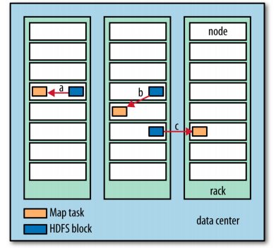
Figure 1: Data-local (a), rack-local (b) and off-rack (c) map tasks
Reduce tasks don’t have the advantage of data-locality; the input to a single reduce task is often the output from all mappers. Therefore the sorted map outputs have to be transferred across the network to the node where the reduce task is running, where they are merged and then passed to the user-defined reduce function.
The number of reduce tasks is not governed by the size of the input, and is specified independently. Twitter does reducer count estimation using hraven.
Hadoop also allows users to specify a combiner function to be run on the map output, to allow users to form input to the reduce function. THis is an optimization: there is no guarantee of how many times it will call the combiner function for a particular map output record. Hence, it should be idempotent.
For example, suppose weather readings for the year 1950 was produced by two maps:
  (1950, 0)
  (1950, 20)
  (1950, 10)

  (1950, 25)
  (1950, 15)
The reduce function (in our case max) would be called with the list:
(1950, [0, 20, 10, 25, 15])
and finally return (1950, 25).
To optimize this, we may have a combiner function that performs max
such that the reduce function would be called with:
(1950, [20, 25])
to produce the same output.
Hadoop uses Unix standard streams as the interface between Hadoop and programs, so any language that can read and write to standard output can be used to write the MapReduce program.
The Hadoop Distributed Filesystem (HDFS)
HDFS is designed for storing very large files with streaming data access patterns, running on clusters of commodity hardware. Hadoop is built around the write-once, read-many-times pattern. Time to read the whole dataset is optimized, over time to read the first record. HDFS is optimized for delivering data at high-throughput, sometimes at the expense of latency. Hence, HDFS is ill-suited for:
- Low-latency file access
- Lots of small files
HDFS Concepts
Block Size
The block size is the minimum amount of data a disk can read or write. HDFS uses a relatively large block size (128MB by default). Unlike a filesystem for a single disk, a file in HDFS that is smaller than a single block does not occupy a full block’s worth of underlying storage. HDFS block sizes are large compared to regular disk blocks to minimize the cost of seeks.
Having a block abstraction for a distributed filesystem brings several benefits. First, it allows a file to be larger than any single disk in the network, since blocks can be stored in any disk. Second, it simplifies the storage subsystem. Third, it fits well with replication, for providing fault tolerance and availability. A block that is unavailable can be replicated from alternative locations.
hadoop fs fsck / -files -blocks
will list the blocks that make up each file in the filesystem.
Namenodes and Datanodes
The HDFS cluster has two types of nodes operating in a master-worker pattern: a namenode (the master) and a number of datanodes (workers). The namenode manages the filesystem namespace. It maintains the filesystem tree, and the metadata for all the files and directories in the tree. This information is persisted in the form of 2 files: the namespace image and the edit log. The namenode knows the datanodes on which all the blocks for a given file are located. This data is not persisted; it is reconstructed from datanodes when the system starts.
A client accesses the filesystem on behalf of the user by communicating with the namenode and datanodes. The filesystem interface is similar to a Portable Operating System Interface (POSIX).
Datanodes store and retrieve blocks when they are told to (by clients or the namenode), and report back to the namenode periodically about the blocks they are storing.
If the namenode is obliterated, all files on the filesystem would be lost, since there is no way to reconstruct the original files, given that this information was stored on the main node. To make the namenode resilient to failure, the files are backed up onto multiple filesystems. A secondary namenode that merges the namespace image with the edit log (to prevent the edit log from growing too large), runs on a separate machine. The state of the secondary namenode always lags behind the primary. Hence, it case of total primary namenode failure, the usual action is to copy the namenode’s metadata files that are on a NFS to secondary, and run the secondary node as the primary.
Block Caching
Frequently accessed blocks may be explicitly cached in the datanode’s memory, in an off-heap block cache. By default, a block is cached only in one datanode’s memory, but this can be configured on a per-file basis. Job schedulers can take advantage of the cached blocks by running tasks on the datanode where the block is cached. A small lookup table used in a join is a good candidate for caching.
HDFS Federation
Introduced in the 2.x release series, HDFS federation allows a custer
to scale by adding namenodes. This is to scale namenodes, which grow
quickly in size because it has to keep a reference to every file and
block in the filesystem. To access a federated HDF cluster, clients
use client-side mount tables to map file paths to namenodes. This is
managed in configuration using ViewFileSystem and the viewfs:// URLs.
Under federation, each namenode manages a namespace volume, which is made up of the metadata for the namespace, and a block pool containing all the blocks for the files in the namespace. Namespace volumes are independent of each other, which means namenodes do not communicate with one another, and failure of one namenode does not affect teh availibility of the namespaces managed by other namenodes. Datanodes register with each namenode in the cluster and store blocks from multiple block pools.
HDFS High Availability
When a namenode fails, recovery can take a long time: an administrator needs to start a new primary namenode, load the namespace image, replay the edit log, and receive block reports from the datanodes.
Hadoop 2 added HDFS high availibility. A pair of namenodes are in active-standby configuration. In the event of failure, the standby namenode takes over as the primary namenode without service interruption.
For this to happen, architectural changes were needed:
- The namenodes must use highly-available shared storage to share the edit log
- Datanodes must send block reports to both namenodes
- Clients must be configured to handle namenode failover
- The secondary namenode’s role is subsumed by the standby, which takes periodic checkpoints of the active namenode’s namespace
There are 2 choices for highly-available shared storage: an NFS filer, or a quorum journal manager (QJM). the QJM is a dedicated HDFS implementation, designed for the sole purpose of a highly available edit log, and is the recommended choice. The QJM runs as a group of journal nodes, and each edit must be written to a majority of the journal nodes. Typically, there are 3 journal nodes, so the system can tolerate the loss of 1 of them. This is similar to the way ZooKeeper works, but QJM does not use ZooKeeper underneath.
Failover and Fencing
The transition from the active namenode to the standby is managed by a new entity in the system called the failover controller. There are various failover controllers but the system called the failover controller. There are varoious failover controllers, but the default implementation uses ZooKeeper to ensure that only one namenode is active. Each namenode runs a lightweight failover controller process whose job is to monitor its namenode for failures and trigger a failover should a namenode fail.
The QJM only allows one namenode to write to the edit log at one time; however, it is still possible for the previously active namenode to serve stale read requests to clients, so setting up an SSH fencing command that will kill the namenode’s process is a good idea. Stronger fencing methods are required with the NFS filer, since it is not possible to only allow one namenode to write at a time.
Client failover is handled transparently by the client library. The simplest implementation uses client-side configuration to control failover.
Hadoop FileSystem Abstractions
HDFS is just one implementation of the filesystem abstraction. There are several implementations, examples of which are listed below:
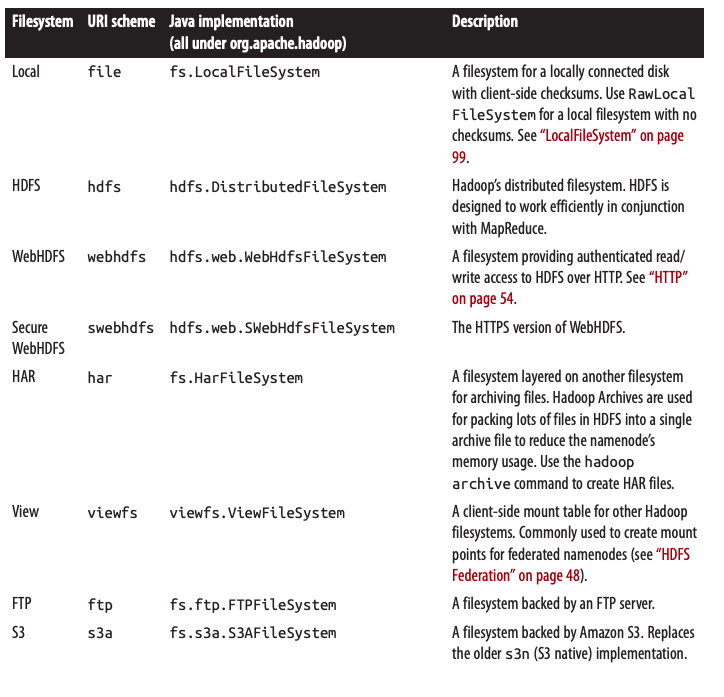
Figure 2: Hadoop filesystems
File writes
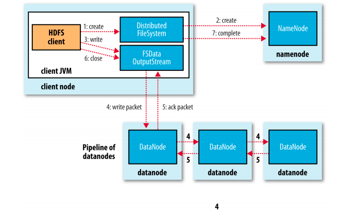
Figure 3: A client writing data to HDFS
Hadoop distcp
distcp is implemented as a MapReduce job where the work of copying is
done by the maps that run in parallel across the cluster. It is an
efficient, distributed copy program.
YARN
Apache YARN is Hadoop’s cluster resource management system. YARN provides APIs for requesting and working with cluster resources, but these APIs are not typically used directly by user code. Instead, users write to higher-level APIs provided by distributed computing frameworks, such as Spark and MapReduce.
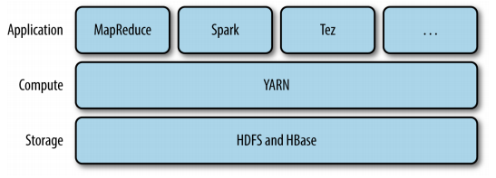
Figure 4: YARN applications
YARN provides its core services via two types of long-running daemon: a resource manager (one per cluster) to manage the use of resources across the cluster, and node managers on all the nodes in the cluster to launch and monitor containers. Depending on how YARN is configured, a container may be a Unix process, or a linux cgroup.
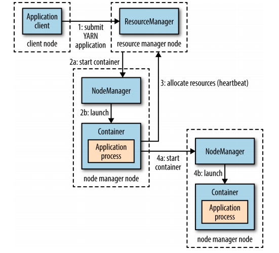
To run an application on YARN, a client contacts the resource manager and asks it to run an application master process. The resource manager finds a node manager that can launch an application master in a container. The application could request more containers from the resource managers, and use them to run a distributed computation. This is what a MapReduce application does. Most non-trivial YARN applications use some form of remote communication to pass status updates and results around, but these are application specific.
Data Serialization
Data is often represented differently in-memory, and requires serialization before being written to disk. For evolvability, serialization formats should provide forward compatibility. This allows schemas to change without affecting data that was written previously. Some serialization formats include:
Thrift and Protocol Buffers are highly similar projects. Thrift is relatively more mature, with generated serialization classes for many different languages, and ships with an RPC framework. Protocol Buffers and gRPC were developed simulataneously, but ship as separate projects.
Avro is designed from the ground-up for the Hadoop filesystem by Doug Cutting, the author of Hadoop. In contrast with Thrift and Protocol Buffers, it provides a dynamic schema. The data format is also splittable by default.
To allow for more efficient reads, Twitter uses Parquet, a project that came out of a collaboration between Twittera and Cloudera. Instead of storing Thrift structures in the Thrift binary format, Parquet uses a data converter to convert Thrift structures into Parquet format, a compressed, columnar data representation.
Kleppmann, n.d.
Parquet’s Columnar Storage
Parquet’s columnar representation is inpired by Google’s Dremel. Melnik et al., n.d.
Thrift and Protocol Buffer’s binary representations are field values laid out sequentially. Using a columnar-striped representation enables queries on just a few columns to read less data from storage.
A key challenge is the natural occurrence of nested records in web and scientific computing. Normalizing these nested records are often computationally too expensive. The approach Dremel takes is storing nested records with their values, and repetition and definition levels.
- Repetition levels
- repetition levels tell us at what repeated field in the field’s path the value has repeated.
- Definition levels
- definition levels tell us how many fields in \(p\) could be undefined, are actually present.
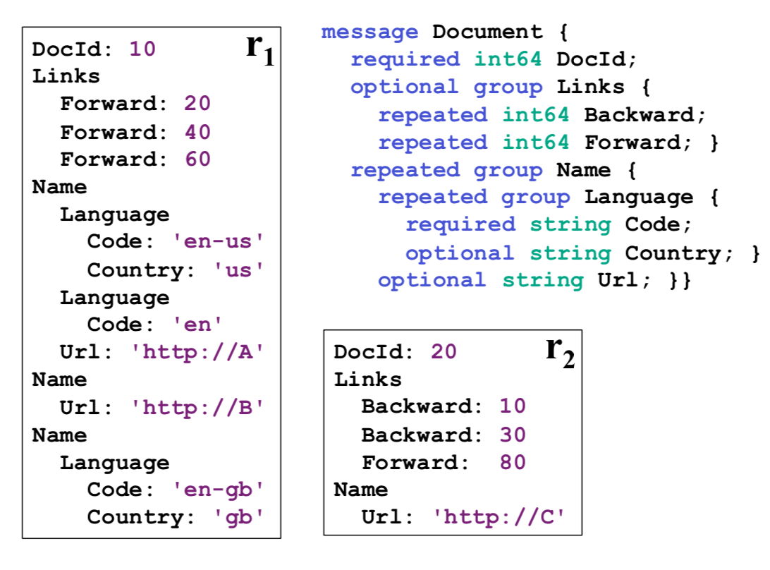
Figure 5: Two sample nested records and their schema
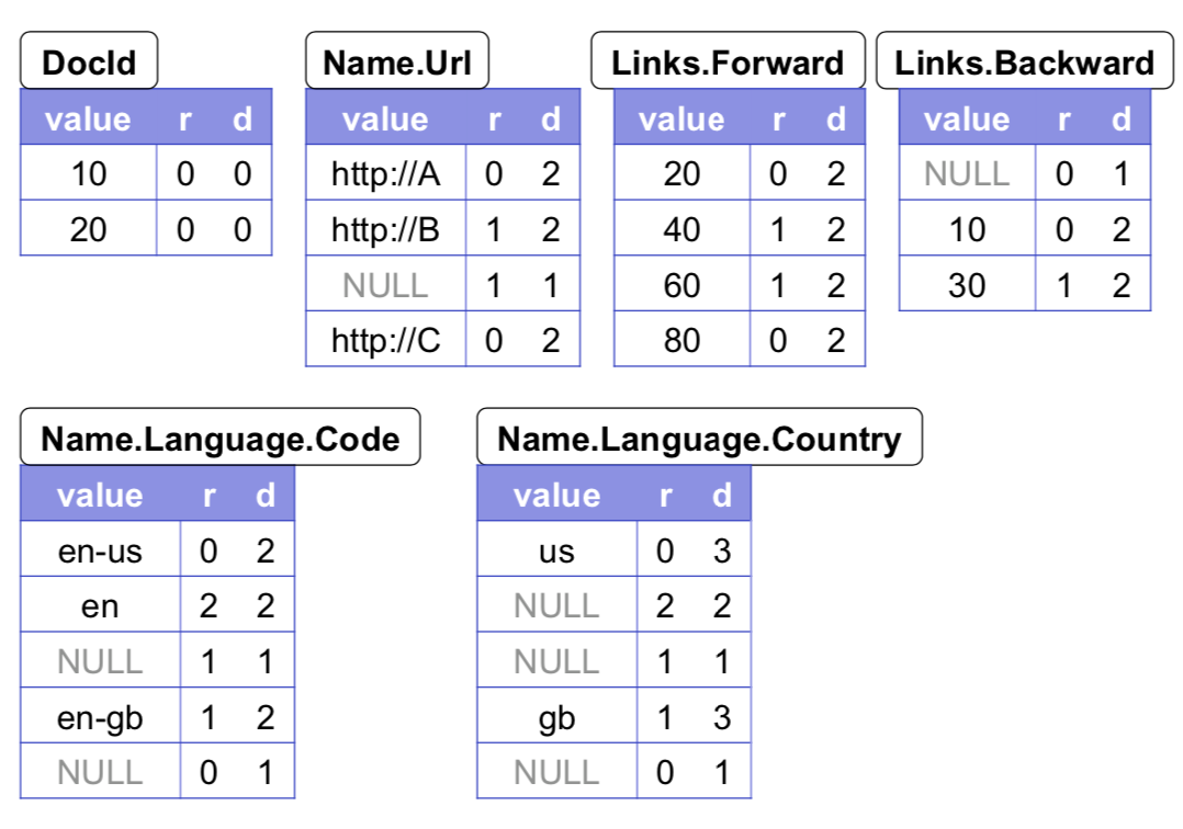
Figure 6: Column-striped representation of the sample data
Each column is stored as a set of blocks, each block containing the repetition and definition levels, and compressed field values.
Record shredding is performed by creating a tree of field writers, whose structure matches the file hierarchy in the schema. Field writers update only when they have their own data, and do not try to propagate the parent state down the tree unless absolutely necessary.
Record assembly is performed by constructing an optimal FSM that reads field values and levels for each field, and append the values sequentially to the output records.
Efficient algorithms for record shredding and assembly are provided in Appendix A of the Dremel paper. Melnik et al., n.d.
Beyond MapReduce
MapReduce - http://research.google.com/archive/mapreduce.html Dataflow model - http://www.vldb.org/pvldb/vol8/p1792-Akidau.pdf FlumeJava - http://research.google.com/pubs/pub35650.html MillWheel - http://research.google.com/pubs/pub41378.html
Beam is an open source, unified model for defining and executing data processing workflows.