Theory Of Computation
Introduction
Finite automata are a useful model for many kinds of important software and hardware. Automatas are found in compilers, software for designing digital circuits, and many more systems.
Grammars provide useful models when designing software that processes data with a recursive structure. The compiler’s parser deals with recursively nested features. Regular Expressions also denote the structure of data, especially in text strings.
The study of automata addresses the following questions:
- What can a computer do?
- What can a computer do efficiently?
Automata theory also provides a tool for making formal proofs, of both the inductive and deductive type.
Formal Proofs
Here the more common proof requirements are here:
- Proving set equivalence: we can approach this by rephrasing it into
an iff statement.
- Prove that if
xis inE, thenxis inF. - Prove that if
xis inF, thenxis inE.
- Prove that if
Inductive Proofs
Suppose we are given a statement \(S(n)\) to prove. The inductive approach involves:
- The basis: where we show \(S(i)\) for a particular \(i\).
- The inductive step: where we show if \(S(k)\) (or \(S(i), S(i+1), \dots, S(k)\)) then \(S(k+1)\).
Structural Inductions
We can sometimes prove statements by construction. This is often the case with recursively defined structures, such as with trees and expressions. This works because we the recursive definition is invoked at each step, so we are guaranteed that at each step of the construction, the construction \(X_i\) is valid.
Automata Theory
Definitions
- alphabet
- An alphabet is a finite, nonempty set of symbols. E.g. \(\Sigma = \{0, 1\}\) represents the binary alphabet
- string
- A string is a finite sequence of symbols chosen from some alphabet. For example, \(01101\) is a string from the binary alphabet. The empty string is represented by ε, and sometimes \(\Lambda\). The length of a string is denoted as such: \(|001| = 3\)
- Powers
- \(\Sigma^k\) represents strings of length \(k\).
- Concatenation
- \(xy\) denotes the concatenation of strings \(x\) and \(y\).
- Problem
- a problem is the question of deciding whether a given string is a member of some particular language.
Finite Automata
An automata has:
- a set of states
- its “control” moves from state to state in response to external inputs
A finite automata is one where the automaton can only be in a single state at once (it is deterministic). Non-determinism allows us to program solutions to problems using a higher-level language.
Determinism refers to the fact that on each input there is one and only one state to which the automaton can transition from its current state. Deterministic Finite Automata is often abbrieviated with DFA.
Deterministic Finite Automata
A dfa consists of:
- A finite set of states, often denoted \(Q\).
- A finite set of input symbols, often denoted \(\Sigma\).
- A transition function that takes as arguments a state and an input symbol and returns a state, often denoted \(\delta\). If \(q\) is a state, and \(a\) is an input symbol, then \(\delta(q,a)\) is that state \(p\) such that there is an arc labeled \(a\) from \(q\) to \(p\).
- A start state, one of the states in \(Q\).
- A set of final or accepting states \(F\). The set \(F\) is a subset of \(Q\).
In proofs, we often talk about a DFA in “five-tuple” notation:
\begin{equation} A = \left(Q, \Sigma, \delta, q_0, F \right) \end{equation}
Simpler Notations
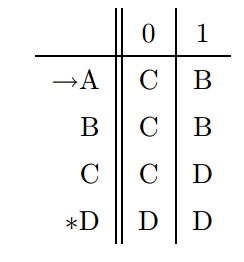
The two preferred notation for describing automata are:
- transition diagrams
- a graph
- transition table
- a tubular listing of the \(\delta\) function, which by implication tells us the states and the input alphabet.
Language of a DFA
We can define the language of a DFA \(A = \left(Q, \Sigma, q_0, F\right)\). This language is denoted \(L(A)\), and is defined by:
\begin{equation} L(A) = \{ w | \delta(q_0, w) \text{ is in } F\} \end{equation}
The language of \(A\) is the set of strings \(w\) that take the start state \(q_0\) to one of the accepting states.
Extending Transition Function to Strings
Basis:
\begin{equation} \hat{\delta}\left(q, \epsilon\right) = q \end{equation}
Induction:
\begin{equation} \hat{\delta}\left(q, xa\right) = \delta \left(\hat{\delta}\left(q, x\right), a \right) \end{equation}
Nondeterministic Finite Automata
A NFA has can be in several states at once, and this ability is expressed as an ability to “guess” something about its input. It can be shown that NFAs accept exactly the regular languages, just as DFAs do. We can always convert an NFA to a DFA, although the latter may have exponentially more states than the NFA.
Definition
An NFA has:
- A finite set of states \(Q\).
- A finite set of input symbols \(\Sigma\).
- A starting state \(q_0 \in Q\),
- A set of final states \(F \subset Q\).
- A transition function that takes a state in \(Q\) and an input symbol in \(\Sigma\) as arguments and returns a subset of \(Q\).
The Language of an NFA
if \(A = (Q, \Sigma, \delta, q_0, F)\) is an NFA, then
\begin{equation} L(A) = \{w | \hat{\delta}(q_0, w) \cap F \neq \emptyset\} \end{equation}
That is, \(L(A)\) is the set of strings \(w\) in \(\Sigma^*\) such that \(\hat{\delta}(q_0, w)\).
The Equivalence of DFA and NFA
Finite Automata with Epsilon-Transitions
Transitions on ε, the empty string, allow NFAs to make a transition spontaneously. This is sometimes referred to as ε-NFAs, and are closely related to regular expressions.
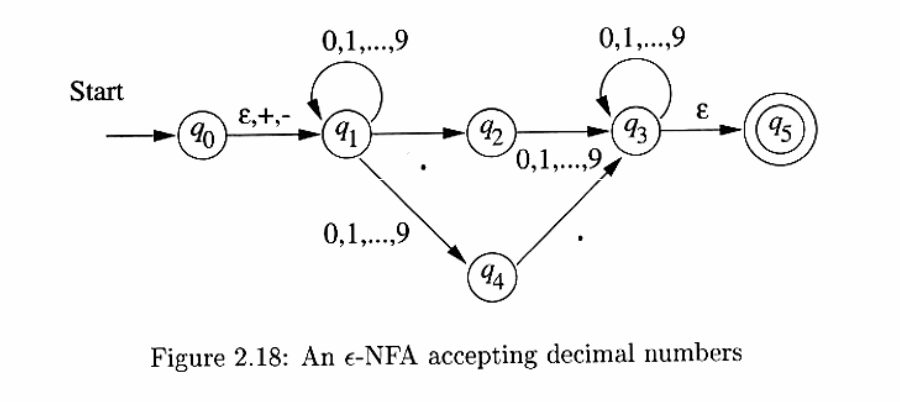
Of particular interest is the transition from \(q_0\) to \(q_1\), where the \(+\) and \(-\) sign is optional.
Epsilon-Closures
We ε-close a state \(q\) by following all transitions out of \(q\) that are labelled ε, eventually finding all states that can be reached from \(q\) along any path whose arcs are all labelled ε.
ε-closure allows us to explain easily what the transitions of an ε-NFA look like when given a sequence of (non-ε) inputs. Suppose that \(E = (Q, \Sigma, \delta, q_0, F)\) is an ε-NFA. We first define \(\hat{\delta}\), the extended transition function, to reflect what happens on a sequence of inputs.
BASIS: \(\hat{\delta}(q, \epsilon) = ECLOSE(q)\). If the label of the path is ε, then we can follow only ε-labeled arcs extending from state \(q\).
INDUCTION: Suppose \(w\) is of the form \(xa\), where \(a\) is the last symbol of \(w\). Note that \(a\) is a member of \(\Sigma\); it cannot be ε. Then:
\begin{align}
\text{Let } & \hat{\delta}(q, x) = \{p_1, p_2, \dots, p_k\} \\\
& \bigcup\limits_{i=1}^k \delta(p_i, a) = \{r_1, r_2, \dots, r_m\} \\\
\text{Then } & \hat{\delta}(q,w) = \bigcup\limits_{j=1}^m ECLOSE(r_j)
\end{align}
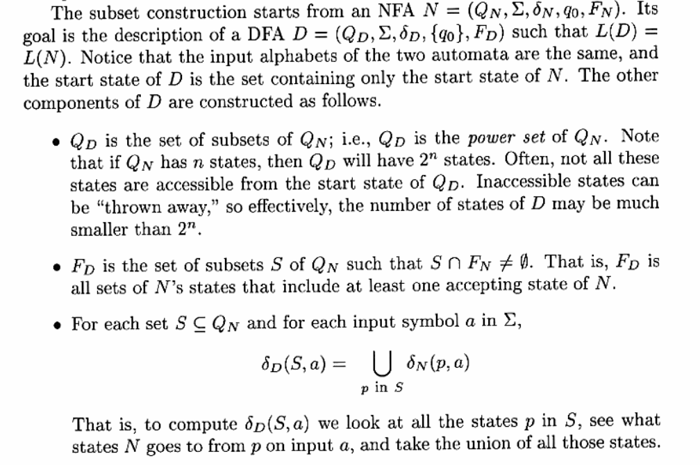
Eliminating ε-Transitions
Given any ε-NFA \(E\), we can find a DFA \(D\) that accepts the same language as \(E\).
Let \(E = (Q_E, \Sigma, \delta_E, q_0, F_E)\), then the equivalent DFA \(D = (Q_D, \Sigma, \delta_D, q_D, F_D)\) is defined as follows:
- \(Q_D\) is the set of subsets of \(Q_E\). All accessible states of \(D\) are ε-closed subsets of \(Q_E\), i.e. \(S \subseteq Q_K s.t. S = ECLOSE(S)\). Any ε-transition out of one of the states in \(S\) leads to another state in \(S\).
- \(q_D = ECLOSE(q_0)\), we get the start state of \(D\) by closing the set consisting of only the start state of \(E\).
- \(F_D\) is those set of states that contain at least one accepting state of \(E\). \(F_D = \{S | S \text{ is in } Q_D \text{ and } S \cap F_E \neq \emptyset \}\)
- \(\delta_D(S,a)\) is computed for all \(a\) in \(\Sigma\) and sets \(S\) in \(Q_D\) by:
- Let \(S = \{p_1, p_2, \dots, p_k\}\)
- Compute \(\bigcup\limits_{i=1}^{k}\delta_E(p_i, a) = \{r_1, r_2, \dots, r_m\}\)
- Then \(\delta_D(S, a) = \bigcup\limits_{j=1}^{m}ECLOSE(r_j)\)
Regular Expressions
Regular expressions may be thought of as a “programming language”, in which many important applications like text search applications or compiler components can be expressed in.
Regular expressions can define the exact same languages that various forms of automata describe: the regular languages. Regular expressions denote languages. We define 3 operations on languages that the operators of regular expressions represent.
- The union of two languages \(L \bigcup M\), is the set of strings that are either in \(L\) or \(M\).
- The concatenation of languages \(L\) and \(M\) is the set of strings that can be formed by taking any string in \(L\) and concatenating it with any string in \(M\).
- The closure (or star, or Kleene closure) is denoted \(L^*\) and represents the set of those strings that can be formed by taking any number of strings from \(L\), possibly with repetitions, and concatenating all of them.
We can describe regular expressions recursively. For each expression \(E\), we denote the language it represents with \(L(E)\).
BASIS:
- The constants \(\epsilon\) and \(\emptyset\) are regular expressions, denoting the languages \(\{\epsilon\}\) and \(\emptyset\) respectively.
- If \(a\) is a symbol, then \(\mathbb{a}\) is a regular expression. This expression denotes the language \(\{a\}\).
INDUCTION:
- \(L(E) + L(F) = L(E) \bigcup L(F)\)
- \(L(EF) = L(E)L(F)\)
- \(L(E^*) = (L(E))^*\)
- \(L((E)) = L(E)\)
Precedence of regular expression operators
The precedence in order of highest to lowest, is:
- star
- dot (note that this operation is associative)
- union (\(\plus\) operator)
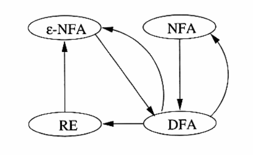
Equivalence of DFA and Regular Expressions
We show this by showing that:
- Every language defined by a DFA is also defined by a regular expression.
- Every language defined by a regular expression is also defined by a $\epilon$-NFA, which we have already shown is equivalent to a DFA.
From DFA to Regular Expression
We can number the finite states in a DFA \(A\) with \(1, 2, \dots, n\).
Let \(R_{ij}^{(k)}\) be the name of a regular expression whose language is the set of strings \(w\) such that \(w\) is the label of a path from state \(i\) to state \(j\) in a DFA \(A\), and the path has no intermediate node whose number is greater than \(k\). To construct the expression \(R_{ij}^{(k)}\), we use the following inductive definition, starting at \(k= 0\), and finally reaching \(k=n\).
BASIS: \(k=0\). Since the states are numbered \(1\) or above, the restriction on paths is that the paths have no intermediate states at all. There are only 2 kinds of paths that meet such a condition:
- An arc from node (state) \(i\) to node \(j\).
- A path of length \(0\) that consists only of some node \(i\).
If \(i \ne j\), then only case \(1\) is possible. We must examine DFA \(A\) and find input symbols \(a\) such that there is a transition from state \(i\) to state \(j\) on symbol \(a\).
- If there is no such symbol \(a\), then \(R_{ij}^{(0)} = \emptyset\).
- If there is exactly one such symbol \(a\), then \(R_{ij}^{(0)} = \mathbb{a}\)
- If there are symbols \(a_1, a_2, \dots, a_k\) that label arcs from state \(i\) to state \(j\), then \(R_{ij}^{(0)} = \mathbb{a_1} + \mathbb{a_2} + \dots + \mathbb{a_k}\)
In case (a), the expression becomes \(\epsilon\), in case (c), the expression becomes \(\epsilon + \mathbb{a_1} + \mathbb{a_2} + \dots + \mathbb{a_k}\).
INDUCTION: Suppose there is a path from state \(i\) to state \(j\) that goes through no state higher than \(k\). Then either:
- The path does not go through state \(k\) at all. In this case, the label of the path is \(R_{ij}^{(k-1)}\).
- The path goes through state \(k\) at least once. We can break the path into several pieces:
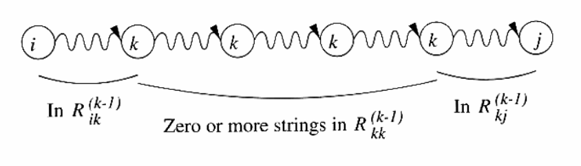
Then the set of labels for all paths of this type is represented by the regular expression \(R_{ik}^{(k-1)}(R_{kk}^{(k-1)})^*R_{kj}^{(k-1)}\). Then, we can combine the expressions for the paths of the two above:
\begin{equation} R_{ij}^{(k)} = R_{ij}^{(k-1)} + R_{ik}^{(k-1)}(R_{kk}^{(k-1)})^*R_{kj}^{(k-1)} \end{equation}
We can compute \(R_{ij}^{(n)}\) for all \(i\) and \(j\), and the language of the automaton is then the sum of all expressions \(R_{ij}^{(n)}\) such that state \(j\) is an accepting state.
Converting DFAs to regular expressions by eliminating states
The above method of conversation always works, but is expensive. \(n^3\) expressions have to be constructed for an n-state automaton, but the length of the expression can grow by a factor of 4 on the average, with each of the \(n\) inductive steps, and the expressions themselves could reach on the order of \(4^n\) symbols.
The approach introduced here avoids duplicating work at some points, by eliminating states. If we eliminate a state \(s\), then all paths that went through \(s\) no longer exist in the automaton. To preserve the language, we must include on an arc that goes directly from \(q\) to \(p\), the labels of paths that went from some state \(q\) to \(p\) through \(s\). This label now includes strings, but we can use a regular expression to represent all such strings.
Hence, we can construct a regular expression from a finite automaton as follows:
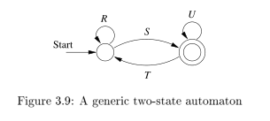
- For each accepting state \(q\), apply the reduction process to produce an equivalent automaton with regular-expression labels on the arcs. Eliminate all states except \(q\) and the start state \(q_0\).
- If \(q \neq q_0\), then a two-state automaton remains, as depicted. The regular expression for the automaton is \((R + SU^*T)^*SU^*\).
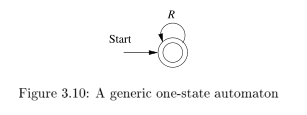
- If the start state is also an accepting state, then we must perform a state-elimination from the original automaton that gets rid of every state but the start state, leaving a one-state automaton, which accepts \(R^*\).
Converting regular expressions to automata
We can show every language defined by a regular expression is also defined by a finite automaton, and we do so by converting any regular expression \(R\) to an $ε$-NFA \(E\) with:
- Exactly one accepting state
- No arcs into initial state
- No arcs out of the accepting state
The proof is conducted by structural induction on R, following the recursive definition of regular expressions.
The basis of the induction involves constructing automatons for regular expressions (a) \(\epsilon\), (b) \(\emptyset\) and (c) \(\mathbb{a}\). They are displayed below:
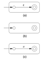
The inductive step consists of 4 cases: (a) The expression is \(R + S\) for some smaller expressions \(R\) and \(S\). (b) The expression is \(RS\) for smaller expressions \(R\) and \(S\). (c) The expression is \(R*\) for some smaller expression \(R\). (d) The expression is (R) for some expression R. The automatons for (a), (b), and (c) are shown below:
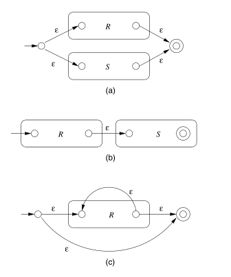
The automaton for \(R\) also serves as the automaton for \(( R)\).
Algebraic law for regular expressions
- commutativity
- \(x + y = y + x\).
- associativity
- \((x \times y) \times z = x \times (y \times z)\).
- distributive
- \(x \times (y + z) = x \times y + x \times z\)
- \(L + M = M + L\)
- \((L + M) + N = L + (M + N)\)
- \((LM)N = L(MN)\)
- \(\emptyset + L = L + \emptyset = L\). \(\emptyset\) is the identity for union.
- \(\epsilon L = L \epsilon = L\). \(\epsilon\) is the identity for concatenation.
- \(\emptyset L = L\emptyset = \emptyset\). \(\emptyset\) is the annihilator for concatenation.
- \(L(M + N) = LM + LN\) (left distributive)
- \((M + N)L = ML + NL\) (right distributive)
- \(L + L = L\) (idempotence law)
- \((L^*)^* = L^*\).
- \(\emptyset^* = \epsilon\)
- \(\epsilon^* = \epsilon\)
- \(L^{+} = LL^* = L^*L\).
- \(L^* = L^{+} + \epsilon\)
- \(L? = \epsilon + L\)
Discovering laws for regular expressions
The truth of a law reduces to the question of the equality of two languages. We show set equivalence: a string in one language must be in another, and vice-versa.
Properties of Regular Languages
Regular languages exhibit the “closure” property. These properties let us build recognizers for languages that are constructed from other languages by certain operations. Regular languages also exhibit “decision properties”, which allow us to make decisions about whether two automata define the same language. This means that we can always minimize an automata to have as few states as possible for a particular language.
Pumping Lemma
We have established that the class of languages known as regular languages are accepted by DFAs, NFAs and by $ε$-NFAs.
However, not every language is a regular language. An easy way to see this is that the number of languages is infinite, but DFAs have finite number of states, and are finite.
The pumping lemma lets us show that certain languages are not regular.
Let \(L\) be a regular language. Then there exists a constant \(n\) (which depends on \(L\)) such that for every string \(w\) in \(L\) such that \(| w | \ge n\), we can break \(w\) into three strings \(w = xyz\) such that:
- \(y \ne \epsilon\)
- \(| xy | \le n\)
- For all \(k \ge 0\), the string \(xy^k z\) is also in \(L\)
That is, we can always find a non-empty string \(y\) not too far from the beginning of \(w\) that can be “pumped”. This means repeating \(y\) any number of times, or deleting it, keeps the resulting string in the language \(L\).
Note that there has been other ways to prove irregularity of languages.
Closure of Regular Languages
If certain languages are regular, then languages formed from them by certain operations are also regular. These are referred to as the closure properties of regular languages. Below is a summary:
- Union of 2 regular languages
- Intersection of 2 regular languages
- Complement of 2 regular languages
- Difference of 2 regular languages
- Reversal of a regular language
- Closure (star) of a regular language
- The concatenation of regular languages
- A homomorphism (substitution of strings for symbols) of a regular language
- The inverse homomorphism of a regular language
The above are all regular.
Context-free Grammars and Languages
Context-free languages are a larger class of languages, that have context-free grammars. We show how these grammars are defined, and how they define languages.
Context-free grammars are recursive definitions. For example, the context-free grammar for palindromes can be defined as:
- \(P \rightarrow \epsilon\)
- \(P \rightarrow 0\)
- \(P \rightarrow 1\)
- \(P \rightarrow 0P0\)
- \(P \rightarrow 1P1\)
There are four important components in a grammatical description of a language:
- There is a finite set of symbols that form the strings of the language. These alphabets are called the terminals, or terminal symbols.
- There is a finite set of variables, or nonterminals or syntactic categories. Each variable represents a language. In the language above, the only variable is \(P\).
- One of the variables represents the language being defined, called the start symbol.
- There is a finite set of productions or rules that represent the
recursive definition of a language. Each production rule consists:
- A variable that is being defined by the production (called the head).
- The production symbol \(\rightarrow\).
- A string of zero or more terminals and variables.
We can represent any CFG as these 4 components, we denote CFG \(G = (V, T, P, S)\).
Derivations using a Grammar
We can apply the productions of a CFG to infer that certain strings are in the language of a certain variable.
The process of deriving strings by applying productions from head to body requires the definition of a new relation symbol, \(\Rightarrow\). Suppose \(G = (V, T, P, S)\) is a CFG> Let \(\alpha A \beta\) be a string of terminals and variables, with \(A\) a variable. That is \(\alpha\) and \(\beta\) are strings in \((V \cup T)^*\), and \(A\) is in \(V\). Let \(A \rightarrow \gamma\) be a production of \(G\). We say that \(\alpha A \beta \Rightarrow_{G} \alpha \gamma B\). If \(G\) is understood, we can omit the subscript.
We may extend the \(\Rightarrow\) relationship to represent zero, one or many derivation steps, similar to the extended transition function.
Leftmost and Rightmost Derivations
In order to restrict the number of choices we have in deriving a string, it is often useful to require that at each step, we replace the leftmost variable by one of its production bodies. Such a derivation is called a leftmost derivation. Leftmost derivations are indicated with \(\Rightarrow_{lm}\) and \(\Rightarrow_{lm}^*\).
Similarly, it is possible to require that at each step the rightmost variable is replaced by one of its bodies. These are called rightmost derivations. These are similarly denoted \(\Rightarrow_{rm}\) and \(\Rightarrow_{rm}^*\).
The language of a Grammar
If \(G = (V, T, P, S)\) is a CFG, then the language of \(G\), denoted \(L(G)\) is the set of terminal strings that have derivations from the start symbol:
\begin{equation} L(G) = \right\{w in T^* | S \Rightarrow_{G}^* w \left\} \end{equation}
Sentential Forms
Derivations from the start symbol produce strings that have a special role. These are called sentential forms. We also denote left-sentential and right-sentential forms for leftmost derivations and rightmost derivations respectively.
Parse Trees
There is a tree representation of derivations, that clearly show how symbols of a terminal string are grouped into substrings, each of which belongs to the language of one of the variables of the grammar. This tree is the data structure of choice when representing the source of a program.
Construction
The parse trees for a CFG \(G\) are trees with the following conditions:
- Each interior node is labeled by variable in \(V\).
- Each leaf is labeled by either a variable, a terminal, or \(\epsilon\). However, if the leaf is labeled \(\epsilon\), then it must be the only child of its parent.
- If an interior node is labeled \(A\), and its children are labeled \(X_1, X_2, \dots, X_k\), respectively from the left, then \(A \rightarrow X_1 X_2 \dots X_k\) is a production in \(P\).
The yield
The yield of the tree is the concatenation of the leaves of the parse tree from the left. This yield is a terminal string (all leaves are labeled either with a terminal or with \(\epsilon\)). The root is labeled by the start symbol.
Inferences and derivations
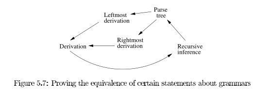
The following statements are equivalent:
- The recursive inference procedure determines that terminal string \(w\) is in the language of variable \(A\).
- \(A \Rightarrow^* w\)
- \(A \Rightarrow_{lm}^* w\)
- \(A \Rightarrow_{rm}^* w\)
- There is a parse tree with root \(A\) and yield \(w\).
We can prove these equivalences using the following arcs:
Linear Grammars
Right linear grammars have all the productions of form:
- \(A \rightarrow wB\) for \(B \in V\) and \(w \in T^*\)
- \(A \rightarrow w\), for \(w \in T^*\)
Every regular language can be generated by some right-linear grammar. Suppose \(L\) is accepted by DFA \(A = (Q, \Sigma, \delta, q_0, F)\), Then, let \(G = (Q, \Sigma, P, q_0)\) where,
- For \(q, p \in Q\), \(a \in \Sigma\), if \(\delta(q, a) = p\), then we have a production in \(P\) of the form \(q \rightarrow ap\).
- We also have productions \(q \rightarrow \epsilon\) for each \(q \in F\).
We can prove by induction on \(|w|\) that \(\hat{\delta}(q_0, w) = p\) iff \(q_0 \Rightarrow^* wp\). This would give \(\hat{\delta}(q_0, w) \in F\) iff \(q_0 \Rightarrow^* w\).
TODO Ambiguous Grammars
Chomsky Normal Form
Chomsky normal form is useful in giving algorithms for working with context-free grammars. A context-free grammar is in Chomsky normal form if every rule is of the form:
- \(A \rightarrow BC\)
- \(A \rightarrow a\)
weher \(a\) is any terminal and \(A\), \(B\), \(C\) are any variables, except \(B\) and \(C\) cannot be the start variable. \(S \rightarrow \epsilon\) is also allowed.
Any context-free language is generated by a context-free grammar in Chomsky normal form. This is because we can convert any grammar into Chomsky normal form.
Pushdown Automata
Pushdown automata are equivalent in power to context-free grammars This equivalence is useful because it gives us two options for proving that a language is context-free. Certain languages are more easily described in terms of recognizers, while others aremore easily described in terms of generators.
Definition
It is in essence a nondeterministic finite automaton with ε-transitions permitted, with one additional capability: a stack on which it can store a string of “stack symbols”.
We can view the pushdown automaton informally as the device suggested below:
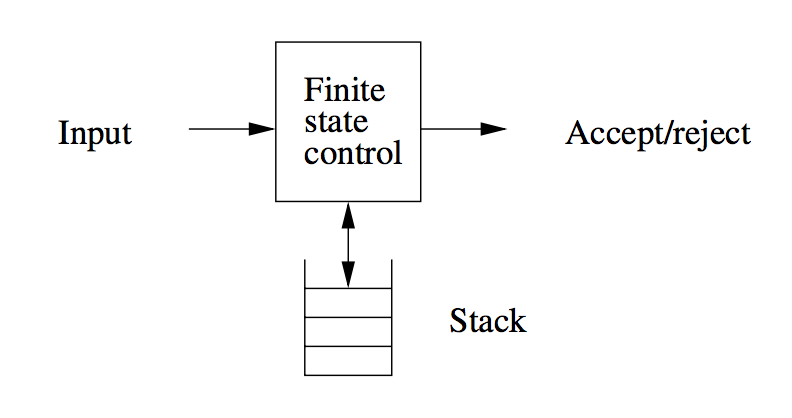
A “finite-state-control” reads inputs, one symbol at a time. The automaton is allowed to observe the symbol at the top of the stack, and to base its transition on its current state. It :
- Consumes from the input the symbol it uses in the transition. If ε is used for the input, then no input symbol is consumed.
- Goes to a new state
- Replaces the symbol at the top of the stack by any string. This corresponds to ε, which corresponds to a pop of the stack. It could also replace the top symbol by one other symbol. Finally the top stack symbol could be replaced by 2 or more symbols, which has the effect of changing the top stack symbol, and pushing one or more new symbols onto the stack.
Formal Definition
We can specify a PDA \(P\) as follows:
\begin{equation} P = (Q,\Sigma, \Gamma, \delta, q_0, Z_0, F) \end{equation}
- \(Q\) is the finite set of states
- \(\Sigma\) is the finite set of input symbols
- \(\Gamma\) is the finite stack alphabet
- \(\delta\) is the transition function, taking a triple $δ(q,a,X), where:
- \(q\) is a state in \(Q\)
- \(a\) is either an input symbol in \(\Sigma\) or \(\epsilon\).
- \(X\) is a stack symbol, that is a member of \(\Gamma\)
- \(q_0\) the start state
- \(Z_0\) the start symbol. Initially, the PDA’s stack consists of this symbol, nothing else
- \(F\) is the set of accepting states
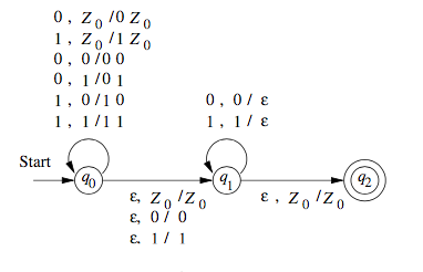
The formal definition of a PDA contains no explicit mechanism to allow the PDA to test for an empty stack. The PDA is able to get the same effect by initially placing a special symbol $ on the stack. If it sees the $ again, it knows that the stack effectively is empty.
We can also draw transition diagrams for PDAs. An example is shown below.
Instantaneous Descriptions
We represent the configuration of a PDA by a triple \((q, w, \gamma)\), where:
- \(q\) is the state.
- \(w\) is the remaining input
- \(\gamma\) is the stack contents
Conventionally, we show the top of the stack at the left, and the bottom at the right. This triple is called the instantaneous description, or ID, of the pushdown automaton.
For finite automata, the \(\hat{\gamma}\) notation was sufficient to represent sequences of instantaneous descriptions through which a finite automaton moved. However, for PDAs we need a notation that describes changes in the state, input and stack. Hence, we define \(\vdash\) as follows. Supposed \(\delta(q, a, X)\) contains \((p, \alpha)\). Then for all stings \(w\) in \(\Sigma^*\) and \(\beta\) in \(\Gamma^*\):
\begin{equation} (q, aw, X\beta) \vdash (p, w, \alpha\beta) \end{equation}
We use \(\vdash^*\) to represent zero or more moves of the PDA.
The Languages of PDAs
The class of languages for PDAs that accept by final state and accept by empty stack are the same. We can show how to convert between the two.
Acceptance by Final State
Let \(P = (Q, \Sigma, \Gamma, \delta, q_0, Z_0, F)\) be a PDA. Then \(L(P)\), the language accepted by P by final state, is:
\begin{equation} \{w | (q_0, w, Z_0) \vdash^* (q, \epsilon, \alpha) \} \end{equation}
for some state \(q\) in \(F\) and any stack string \(\alpha\).
Acceptance by Empty Stack
Let \(P = (Q, \Sigma, \Gamma, \delta, q_0, Z_0, F)\) be a PDA. We define \(N(P) = \{w | (q_0, w, Z_0) \vdash^* (q, \epsilon, \epsilon)\}\). That is \(N(P)\) is the set of inputs \(w\) that \(P\) can consume and at the same time empty its stack.
From Empty Stack to Final State
Theorem:
If \(L = N(P_N)\) for some PDA \(P_N\), then there is a PDA \(P_F\) such that \(L = L(P_F)\).
Proof:
We use a new symbol \(X_0\), not a symbol of \(\Gamma\); \(X_0\) is both the start symbol of \(P_F\) and a marker on the bottom of the stack that lets us know when \(P_N\) has reached an empty stack, then it knows that \(P_N\) would empty its stack on the same input.
We also use a new start state \(p_0\), whose sole function is to push \(Z_0\), the start symbol of \(P_N\), onto the top of the stack and enter \(q_0\), the start state of \(P_N\). \(P_F\) simulates \(P_N\), until the stack of \(P_N\) is empty, which \(P_F\) detects because it sees \(X_0\) on the top of the stack.
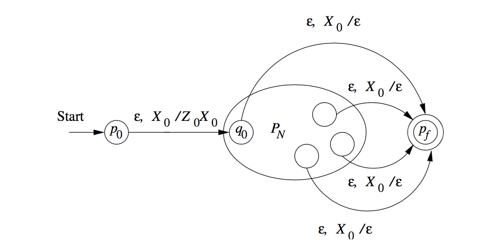
Hence, we can specify \(P_F = (Q \cup \{p_0, p_f\}, \Sigma, \Gamma \cup \{X_0\}, \delta_F, p_0, X_0, \{p_f\}\):
- \(\delta_F(p_0, \epsilon, x_0) = \{(q_0, Z_0, X_0\}\).
- For all states \(q\) in \(Q\), inputs \(a\) in \(\Sigma\) or \(a = \epsilon\), and the stack symbols \(Y\) in \(\Gamma\), \(\delta_F(q,a,Y)\) contains all the pairs in \(\delta_N(qa,Y)\).
- \(\delta_F(q, \epsilon, X_0\) contains \((p_f, \epsilon)\) iff w is in \(N(P_N)\).
From Final State to Empty Stack
Whenever \(P_F\) enters an accepting state after consuming input \(w\), \(P_N\) will empty its stack after consuming \(w\).
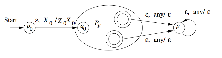
To avoid simulating a situation where \(P_F\) accidentally empties its stack without accepting, \(P_N\) also utilizes a marker \(X_0\) on the bottom of its stack.
That is \(P_N = (Q \cup \{p_0, p\}, \Sigma, \Gamma \cup \{X_0\}, \delta_N, p_0, X_0)\), where \(\delta_N\) is:
- \(\delta_N(p_0, \epsilon, x_0) = \{(q_0, Z_0, X_0)\}\)
- For all states \(q\) in \(Q\), input symbols \(a\) in \(\Sigma\) or \(a = \epsilon\), \(Y\) in \(\Gamma\), \(\delta_N(q, a, Y)\) contains every pair that is in \(\delta_F(q, a Y)\).
- For all accepting states \(q\) in \(F\), and stack symbols \(Y\) in \(\Gamma\) or \(Y = X_0\), \(\delta_N(q, \epsilon, Y)\) contains \((p, \epsilon)\). Whenever \(P_F\) accepts, \(P_N\) can start emptying its stack without consuming any input.
- For all stack symbols \(Y\) in \(\Gamma\) or \(Y = X_0\), \(\delta_N(p, \epsilon, Y) = \{(p, \epsilon)\}\). Once in state \(p\), which only occurs when \(P_F\) is accepted, \(P_N\) pops every symbol on its stack, until the stack is empty.
Equivalence of CFG and PDA
Let \(A\) be a CFL. From the definition we know that \(A\) has a CFG, \(G\), generating it. We show how to convert \(G\) into an equivalent PDA.
The PDA \(P\) we now describe will work by accepting its input \(w\), if \(G\) generates that input, by determining whether there is a derivation for \(w\). Each step of the derivation yields an intermediate string of variables and terminals. We design \(P\) to determine whether some series of substitutions of \(G\) can lead from the start variable to \(w\).
The PDA \(P\) begins by writing the start variable on its stack. It goes through a series of intermediate strings, making one substitution after another. Eventually it may arrive at a string that contains only terminal symbols, meaning that it has used the grammar to derive a string. Then \(P\) accepts if this string is identical to the string it has received as input.
- Place the marker symbol $ and the start variable on the stack
- Repeat:
- If the top of stack is a variable symbol \(A\), nondeterministically select one of the rules for \(A\) and substitute \(A\) by the string on the right-hand side of the rule
- If the top of stack is a terminal symbol \(a\), read the next symbol from the input and compare it to \(a\). If they match, continue. Else, reject the branch of nondeterminism.
- If the top of stack is the symbol $, enter the accept state.
Now we prove the reverse direction. We have a PDA \(P\) and want to make a CFG \(G\) that generates all the strings that \(P\) accepts.
For each pair of states \(p\) and \(q\), the grammar will have a variable \(A_{pq}\).
First, we simplify the task by modifying P slightly to give it the following three features.
- It has a single accept state, \(q_{accept}\).
- It empties its stack before accepting.
- Each transition either pushes a symbol onto the stack (a push move) or pops one off the stack (a pop move), but it does not do both at the same time.
Giving \(P\) features 1 and 2 is easy. To give it feature 3, we replace each transition that simultaneously pops and pushes with a two transition sequence that goes through a new state, and we replace each transition that simultaneously pops and pushes with a two transition sequence that goes through a new state, and we replace each transition that neither pops nor pushes with a two transition sequence that pushes then pops an arbitrary stack symbol.
To design \(G\) so that \(A_{pq}\) generates all strings that take \(P\) from \(p\) to \(q\), regardless of the stack contents at \(p\), leaving the stack at \(q\) in the same condition as it was at \(p\).
First, we simplify our task by modifying \(P\) slightly to give it the following three features.
Deterministic Pushdown Automata
DPDAs accept a class of languages between the regular languages and the CFLs.
We can easily show that DPDAs accept all regular languages by making it simulate a DFA (ignoring the stack).
While DPDAs cannot represent all CFLs, it is able to represent languages that have unambiguous grammars.
Properties of Context-Free Languages
Simplification of CFG
The goal is to reduce all CFLs to Chomsky Normal Form. To get there, we must make several preliminary simplifications, which are useful in their own ways.
-
Elimination of useless symbols
- Remove all non-reachable symbols: starting from \(S\), if it is impossible to reach a symbol, then it is non-reachable and can be removed. Example: \(S \rightarrow a, B \rightarrow b\), then \(B\) is not reachable.
- Remove all non-generating symbols: for each symbol, check if the symbol can ever generate a terminating string. If not, remove it. Example: \(A \rightarrow A | Ab\), \(A\) is non-generating and can be removed.
- It is important to remove non-generating symbols first, because it can lead to more non-reachable symbols.
-
Removal of unit productions
-
Unit productions look like \(A \rightarrow B\). We do unit production elimination to get a grammar into Chomsky Normal form.
-
To eliminate unit productions, we substitute the unit symbol into the production.
-
-
Removal of \(\epsilon\) productions
- Start from any symbol, remove the \(\epsilon\) production, by substituting all possibilities. E.g. \(S \rightarrow AB | AC\), and we eliminate $ε$-productions from \(B\): \(S \rightarrow AB | A | AC\).
- Eliminate until no more $ε$-productions.
- When an $ε$-production is eliminated from a symbol, it does not need to be reapplied if it appears again in the same symbol.
-
Conversion to Chomsky Normal Form
After performing the preliminary simplifications, we can then:
- Arrange that all bodies of length 2 or more consist only of variables
- Break bodies of length 3 or more into a cascade of productions
Pumping Lemma for CFLs
In any sufficiently long string in a CFL, it is possible to find at most 2 short, nearby substrings, that we can pump in tandem. First, we use several results, that we will state below.
- Conversion to CNF converts a parse tree into a binary tree.
- For a CNF grammar \(G = (V, T, P, S)\), if the length of the longest path is \(n\), then \(|w| \le 2^{n-1}\) for all terminal strings \(w\).
Let \(L\) be a CFL. Then there exists a constant \(n\) (which depends on \(L\)) such that for every string \(z\) in \(L\) such that \(| z | \ge n\), we can break \(z\) into three strings \(z = uvwxy\) such that:
- $ vx ≠ ε$
- \(| vwx | \le n\)
- For all \(i \ge 0\), the string \(uv^i wx^i y\) is also in \(L\)
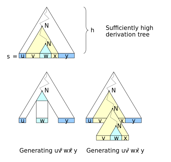
If \(s\) is sufficiently long, its derivation tree w.r.t. a Chomsky normal form grammar must contain some nonterminal \(N\) twice on some tree path (upper picture). Repeating \(n\) times the derivation part \(N \Rightarrow \dots \Rightarrow vNx\) obtains a derivation for \(u v^n w x^n y\).
Closure Properties of CFLs
First, we introduce the notion of substitutions. Let \(\Sigma\) be an alphabet, and suppose that for every symbol \(a\) in \(\Sigma\), we choose a language \(L_a\). These chosen languages can be over any alphabets, not necessarily \(\Sigma\) and not necessarily the same. The choice of languages defines a function \(s\) on \(\Sigma\), and we shall refer to \(L_a\) as \(s(a)\) for each symbol \(a\).
If \(w = a_1 a_2 \dots a_n\) in \(\Sigma^*\), then \(s(w)\) is the language of all strings \(x_1 x_2 \dots x_n\) such that the string \(x_i\) is in the language \(s(a_i)\). \(s(L)\) is the union of \(s(w)\) for all strings \(w\) in \(L\).
The substitution theorem states that if we can find a substitution function \(a\) on a CFL, then the resultant language \(s(a)\) is also a CFL.
CFLs are closed under:
- Union
\(L_1 \cup L_2\) is the language \(s(L)\), where \(L\) is the language \(\{1, 2\}\), and \(s(1) = L_1\) and \(s(2) = L_2\).
- Concatenation
\(L_1 L_2\) is the language \(s(L)\), \(L = {12}\), and \(s(1) = L_1\) and \(s(2) = L_2\).
- Closure, and positive closure (asterisk and plus)
\(L\) is the language \({1}^*\), and \(s\) is the substitution \(s(1) = L_1\), then \(L_1^* = s(L)\). Similarly, for positive closure, \(L = \{1\}^+\) and \(L_1^+ = s(L)\).
- Homomorphism
\(s(a) = \{h(a)\}\), for all \(a\) in \(\Sigma\). Then \(h(L) = s(L)\).
These are the base closure properties. CFLs are also closed under reversal. We can prove this by constructing a grammar for the reversed CFL.
CFLs are not closed under intersection. However, CFLs are closed under the operation of “intersection with a regular language”. To prove this, we use the PDA representation of CFLs, and FA representation of regular languages. We can run the FA in parallel with the PDA.
CFLs are also closed under inverse homomorphism. The proof is similar to that of regular languages, but using a PDA, but is more complex because of the stack introduced in the PDA.
Decision Properties of CFLs
First, we consider the complexity of converting from a CFG to a PDA, and vice versa. Let \(n\) be the length of the entire representation of a PDA or CFG.
Below, we list algorithms linear in the size of the input:
- Converting a CFG to a PDA
- Converting a PDA that accepts by final state to one that accepts by empty stack
- Converting a PDA that accepts by empty stack to one that accepts by final state
The running time of conversion from a PDA to a grammar is much more complex. The upper bound on the number of states and stack symbols is \(n^3\), so there cannot be more than \(n^3\) variables of the form \([pXq\) constructed for the grammar. However, the running time of conversion could still be exponential because there are no limits to the number of symbols put on the stack.
However, we can break the pushing of a long string of stack symbols into a sequence of at most \(n\) steps that each pushes one symbol. Then each transition has no more than 2 stack symbols, and the total length of all the transition rules has grown by at most a constant factor, i.e. it is still \(O(n)\). There are \(O(n)\) transition rules, and each generates \(O(n^2)\) productions, since there are only 2 states that need to be chosen in the productions that come from each rule. Hence, the constructed grammar has length \(O(n^3)\), and can be constructed in cubic time.
Running Time of Conversion to CNF
- Detecting reachable and generating symbols can be done in \(O(n)\) time, and removing useless symbols takes \(O(n)\) time and does not increase the size of the grammar
- Constructing unit pairs and eliminating unit productions takes \(O(n^2)\) time, and results in a grammar whose length is \(O(n)\).
- Replacing terminals by variables in production bodies takes \(O(n)\) time and results in a grammar whose length is \(O(n)\).
- Breaking production bodies of length 3 or more takes \(O(n)\) time and results in a grammar of length \(O(n)\).
However eliminating $ε$-productions is tricky. If we have a production body of length \(k\), we can construct from that one production \(2^{k-1}\) productions for the new grammar, so this part of the construction could take \(O(2^n)\) time. However, we can break all long production bodies into a sequence of productions with bodies of length 2. This step takes \(O(n)\) time and grows only linearly, and makes eliminating $ε$-productions run in \(O(n)\) time.
In all, converting to CNF form is a \(O(n^2)\) algorithm.
Testing for emptiness of CFL
This is equivalent to testing if \(S\) is generating. The algorithm goes as follows:
We maintain an array indexed by variable, which tells whether or not we have established that a variable is generating.For each variable there is a chain of all the positions in which the variable occurs (solid lines). The dashed lines suggest links from the productions to their counts.
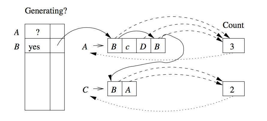
For each production, we count the number of positions holding variables whose ability to generate is not yet accounted for. Each time the count for a head variable reaches 0, we put the variable on a queue of generating variables whose consequences need to be explored.
This algorithm takes \(O(n)\) time:
- There are at most \(n\) variables in a grammar of size \(n\), creation and initialization of the array can be done in \(O(n)\) time.
- Initialization of the links and counts can be done in \(O(n)\) time.
- When we discover a production has count 0:
- Discover a production has count \(0\), finding which variable is at the head, checking whether it is already known to be generating, and putting it on the queue if not. All these steps are \(O(1)\) for each production so \(O(n)\) in total.
- work done when visiting the production bodies that have the head variable \(A\). This work is proportional to the number of positions with \(A\). Hence, \(O(n)\).
Testing Membership in a CFL
First, we can easily see that algorithms exponential in \(n\) can decide membership. We can convert the grammar to CNF form. As the parse trees are binary trees, there will be exactly \(2n-1\) nodes labeled by variables in the tree for a string \(w\) of length \(n\). The number of possible trees and node-labelings is only exponential in \(n\).
Fortunately, more efficient techniques exist, based on the idea of dynamic programming. Once such algorithm is the CYK Algorithm.
We construct a triangular table, and begin the fill the table row-by-row upwards. The horizontal axis corresponds to the positions of the string \(w = a_1 a_2 \dots a_n\), and the table entry \(X_ij\) is the set of variables $A such that \(A \overset{*}{\Rightarrow} a_i a_{i+1} \dots a_j\). We are interested in whether \(S\) is in the set \(X_{1n}\).
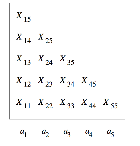
It takes \(O(n)\) time to compute any one entry of the table. Hence, the table-construction process takes \(O(n^3)\) time.
The algorithm for computing \(X_{ij}\) is as such:
BASIS: We compute the first row as follows. Since the string beginning and ending at position \(i\) is just the terminal \(a_i\), and the grammar is in \(CNF\),the only way to derive the string \(a_i\) is to use a production of the form \(A \rightarrow a_i\). Hence \(X_ii\) is the set of variables \(A\) such that \(A \rightarrow a_i\) is a production of \(G\).
INDUCTION: To compute \(X_{ij}\) that is in row \(j - i + 1\), we would have computed all the \(X\) in the rows below i.e. we know about all strings shorter than \(a_i a_{i+1} \dots a_j\), and we know all the proper prefix and proper suffixes of that string.
For \(A\) to be in \(X_{ij}\), we must find variables \(B\), \(C\), and integer \(k\) such that:
- \(i \le k < j\)
- \(B\) is in \(X_{ik}\)
- \(C\) is in \(I_{k+1,j}\)
- \(A \rightarrow BC\) is a production of \(G\)
Finding such variables \(A\) requires us to compare at most \(n\) pairs of previously computed sets. Hence it can be done in \(O(n)\) time.
Turing Machines
We now look at what languages can be defined by any computational device. The Turing Machine is an accurate model for what any physical computing device is capable of doing. More technically, turing machines facilitate proving everyday questions to be undecidable or intractable.
Turing machines are finite automata with a tape of infinite length on which it may read and write data. The machine consists of a finite control, which can be in any of a finite set of states. There is a tape divided into squares or cells; each cell can hold any one of a finite number of symbols.
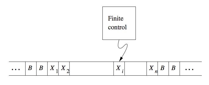
Figure 1: A Turing Machine
Initially, the input, which is a finite-length string of symbols chosen from the input alphabet, is placed on the tape. All other tape cells, extending infinitely to the left and right, initially hold a special symbol called the blank. The blank is a tape symbol, but not an input symbol, and there may be other tape symbols.
There is a tape head that is always positioned at one of the tape cells. The Turing machine is said to be scanning that cell.
A move of the Turing machine is a function of the state of the finite control and the tape symbol scanned.
- Change state: The next state optionally may be the same as the current state.
- Write a tape symbol in the cell scanned. This tape symbol replaces whatever symbol was in that cell.
- Move the tape head left or right.
Formal Notation
The formal notation used for a Turing Machine (TM) is by a 7-tuple:
\begin{equation} M = (Q, \Sigma, \Gamma, \delta, q_0, B, F) \end{equation}
where:
- Q
- The finite set of states of the finite control
- Σ
- The finite set of input symbols
- Γ
- The complete set of tape symbols. Σ is a subset of Γ.
- δ
- The transition function. The arguments of \(\delta(q, X)\) are a state \(q\) and a tape symbol \(X\). The value of \(\delta(q, X)\) is a triple \((p, Y, D)\) where \(p\) is the next state, \(Y\) is the symbol in \(\Gamma\) written in the cell being scanned, \(D\) is a direction, either left or right.
- q_0
- The start state, a member of Q
- B
- the blank symbol, in Γ but not Σ
- F
- the set of final or accepting states
Instantaneous Descriptions
We use the string \(X_1 X_2 \dots X_{i-1} q X_i X_{i+1} \dots X_n\) to represent an ID in which:
- \(q\) is the state of the Turing machine.
- The tape head is scanning the $i$th symbol from the left.
- \(X_1 X_2 \dots X_n\) is the portion of the tape between the leftmost and the rightmost nonblank. As an exception, if the head is to the left of the leftmost nonblank, or to the right of the rightmost nonblank, then some prefix or suffix of \(X_1 X_2 \dots X_n\) will be blank, and \(i\) will be 1 or n, respectively.
We describe moves of a Turing machine \(M = (Q, \Sigma, \Gamma, \delta, q_0, B, F)\) by the \(\vdash\) notation that was used for PDAs. Suppose \(\delta(q, X_i) = (p, Y, L)\). Then \(X_1 X_2 \dots X_{i-1} q X_{i+1} \dots X_n \vdash X_1 X_2 \dots X_{i-2} p X_{i-1} Y X_{i+1} \dots X_n\).
There are 2 important exceptions, when \(i=1\) and M moves to the blank to the left of \(X_1\) and when \(i=n\) and \(Y=B\).
Transition Diagrams
Turing machines can be denoted graphically, as with PDAs.
An arc from state \(q\) to state \(p\) is labelled by one or more items of the form \(X/YD\), where \(X\) and \(Y\) are tape symbols, and \(D\) is a direction from either \(L (\leftarrow)\) or \(R (\rightarrow)\).
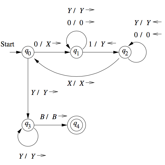
Figure 2: Transition diagram for TM accepting \(0^n 1^n\)
The Language of a TM
\(L(M)\) is the set of strings \(w\) in \(\Sigma^*\) such that \(q_0 w \vdash \alpha p \beta\) for some state in \(p\) in \(F\) and any tape strings \(\alpha\) and \(\beta\). The set of languages we can accept using a TM is often called the recursively enumerable languages or RE languages.
Turing machines and halting
A TM halts if it enters a state \(q\), scanning a tape symbol \(X\), and there is no move in this situation: \(\delta(q, X)\) is undefined. This is another notion of “acceptance”. We can assume that a TM halts if it accepts. That is, without changing the language accepted, we can make \(\delta(q, X)\) undefined whenever \(q\) is an accepting state. However, it is not always possible to require that a TM halts even if it does not accept.
Languages that halt eventually, regardless of whether they accept, are called recursive. If an algorithm to solve a given problem exists, then we say the problem is decidable, so TMs that always halt figure importantly into decidability theory.
Programming Techniques for Turing Machines
Storage in the State
We can use the finite control not only to represent a position in the “program” of a TM, but to hold a finite amount of data. We extend the state as a tuple \([q, A, B, C]\), and having multiple tracks.
Multiple Tracks
One can also think of the tape of a Turing machine as composed of several tracks. Each track can hold one symbol, and the tape alphabet of the TM consists of tuples, with each component for each “track”. A common use of multiple tracks is to treat one track as holding the data, and another track as holding a mark. We can check off each symbol as we “use” it, or we can keep track of a small number of positions within the data by only marking these positions.
Subroutines
A Turing machine subroutine is a set of states that perform some useful process. This set of states includes a start state and another state to pass control to whatever other set of states called the subroutine. Since the TM has no mechanism for remembering a “return address”, that is, a state to go to after it finishes, should our design of a TM call for one subroutine to be called from several states, we can make copies of the subroutine, using a new set of states for each copy. The “calls” are made to the start states of different copies of the subroutine, and each copy “returns” to a different state.
Multitape Turing Machines
The device has a finite control (state), and some finite number of tapes. Each tape is divided into cells, and each cell can hold any symbol of the finite tape alphabet.
Initially, the head of the first tape is at the left end of the input, but all other tape heads are at some arbitrary cell.
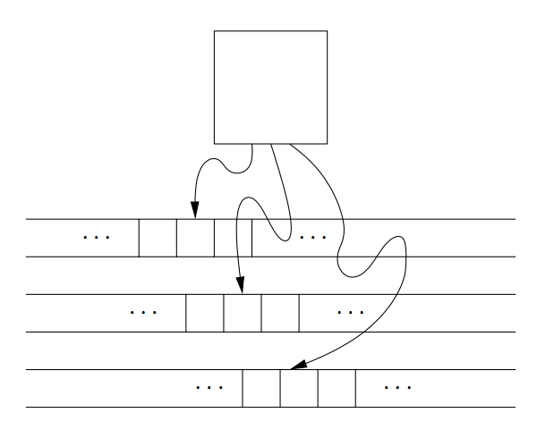
Figure 3: A multitape Turing machine
A move on the multitape TM depends on the state and symbol scanned by each of the tape heads. On each move:
- the control enters a new state, which could be the same as a previous state.
- On each tape, a new tape symbol is written on the cell scanned. This symbol could be the same as the previous symbol.
- Each tape head makes a move, which can be either left, right or stationary.
Equivalence of one-tape and multitape TMs
Suppose language \(L\) is accepted by a k-tape TM \(M\). We simulate \(M\) with a one-tape TM \(N\) whose tape we think of as having 2k tracks. Half of these tracks hold the tapes of \(M\), and the other half of the tracks each hold only a single marker that indicates where the head for the corresponding tape of \(M\) is currently located.
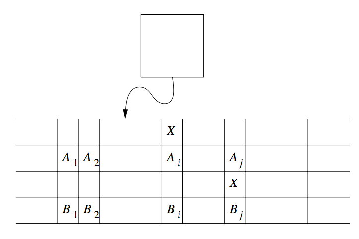
Figure 4: Simulation of two-tape Turing machine by a one-tape Turing machine
To simulate a move of \(M\), \(N\)‘s head must visit the \(k\) head markers. So that \(N\) does not get lost, it must remember how many head markers are to its left at all times. That count is stored as a component of \(N\)‘s finite control. After visiting each head marker and storing the scanned symbol in a component of the finite control, \(n\) knows what tape symbols have been scanned by each of \(M\)‘s heads. \(N\) also knows the state of \(M\), which it stores in \(N\)‘s own finite control. Thus, \(N\) knows what move \(M\) will make.
\(N\) can now revisit each of the head markers on its tape, changing the symbol in the track representing the corresponding tapes of \(M\), and move the head markers left or right, if necessary. \(N\)‘s accepting states are all the states that record \(M\)‘s states as one of the accepting states of \(M\). When the simulated \(M\) accepts, \(N\) also accepts, and \(N\) does not accept otherwise.
The time taken by the one-tape TM \(N\) to simulate \(n\) moves of the k-tape TM \(M\) is \(O(n^2)\).
Non-deterministic Turing Machines
A NTM differs from the deterministic variety by having a transition \(\delta\) such that for each state \(q\) and tape symbol \(X\), \(\delta(q,X)\) is a set of triples \(\{(q_1, Y_1, D_1), \dots, (q_k, Y_k, D_k)\}\).
The NTM can choose at each step any of the triples to be the next move. We can show that NTM and TM are equivalent. The proof involves showing that for every NTM \(M_N\), we can construct a DTM \(M_D\) that explores the ID’s that \(M_N\) can reach by any sequence of its choices. If \(M_D\) has an accepting state, then \(M_D\) enters an accepting state of its own. \(M_D\) must be systematic, putting new ID’s on a queue, rather than a stack, so \(M_D\) would have simulated all sequences up to k moves of \(M_N\) after some finite time.
\(M_D\) is designed as a multi-tape TM. The first tape of \(M_D\) holds a sequence of ID’s of \(M_N\), including the state of \(M_N\). One ID of \(M_N\) is marked as the current ID, whose successor ID’s are in the process of being discovered. All IDs to the left of the current one have been explored and can be ignored subsequently.
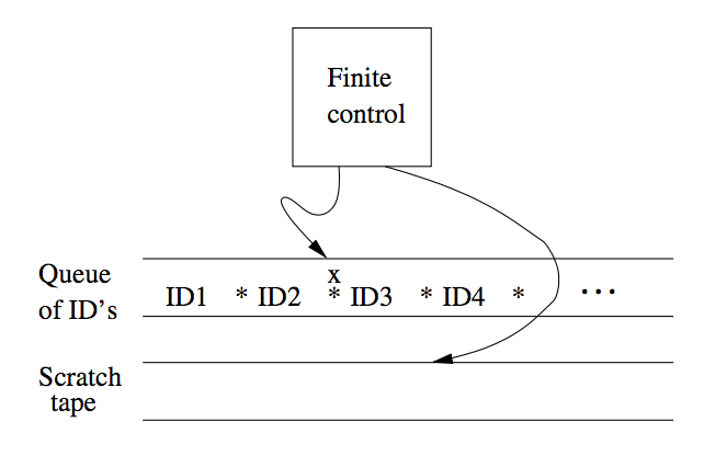
Figure 5: Simulation of NTM by a DTM
To process the current ID, \(M_D\) does:
- \(M_D\) examines the state and scanned symbol of the current ID. Built into the finite control of \(M_D\) is the knowledge of what choices of move \(M_N\) has for each state and symbol. If the state in the current ID is accepting, then \(M_D\) accepts and simulates \(M_N\) no further.
- However, if the state is not accepting, and the state-symbol combination has \(k\) moves, then \(M_D\) uses its second tape to copy the ID and the make k copies of that ID at the end of the sequence of ID’s on tape 1.
- \(M_D\) modifies each of those k ID’s according to a different one of the k choices of move that \(M_N\) has from its current ID.
- \(M_D\) returns to the marked current ID, erases the mark and moves to the next ID to the right. The cycle the repeats with step (1).
This can be viewed as a breadth-first search on all possible IDs reached.
Restricted Turing Machines
Turing Machines with Semi-infinite Tapes
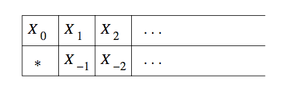
We can assume the tape to be semi-infinite, having no cells to the left of the initial head position, an still retain the full power of TMs.
The trick behind the construction is to use two tracks on the semi-infinite tape. The upper track represents the cells of the original TM that are at or to the right of the initial head position, but in reverse order. The upper track represents \(X_0 , X_1 \dots\) where \(X_0\) is the initial position of the head; \(X_1, X_2\) so on are the cells to its right. The \(*\) on the leftmost cell bottom track serves as an end marker and prevents the head of the semi-infinite TM from falling off the end of the tape.
Another restriction we make is to never write a blank. This combined with the semi-infinite tape restriction means that the tape is at all times a prefix of non-blank symbols followed by an infinity of blanks.
We can construct an equivalent TM \(M_2\) from a TM \(M_1\) by restricting that \(M_1\) never writes a blank, by creating a new tape symbol \(B’\) that functions as a blank, but is not the blank \(B\).
Multistack Machines
A $k$-stack machine is a deterministic PDA with \(k\) stacks. The multistack machine has a finite control, which is in one of a finite state set of states. A move of the multistack machine is based on:
- The state of the finite control
- The input symbol read, which is chosen from the finite input alphabet.
Each move allows the multistack machine to:
- Change to a new state
- Replace the top symbol of each stack with a string of zero or more stack symbols.
If a language is accepted by a TM, it is also accepted by a two-stack machine.
Counter Machines
Counter machines have the same structure as the multistack machine, but in place of each stack is a counter. Counters holdd any non-negative integer, but we can only distinguish between zero and non-zero counters. That is, the move of the counter machine depends on its state, input symbol, and which, if any, of the counters are zero.
Each move can:
- Change state
- Add or subtract 1 from any of its counters independently
A counter machine can be thought of as a restricted multistack machine, where:
- There are only 2 stack symbols, which is the bottom-of-stack marker \(Z_0\), and \(X\).
- \(Z_0\) is initially on each stack.
- We may replace \(Z_0\) only with \(X^i Z_0\), \(i \ge 0\).
- We may replace \(X\) only with \(X^i\), \(i \ge 0\).
We observe the following properties:
- Every language accepted by a counter machine is recursively enumerable.
- Every language accepted by a one-counter machine is a CFL. This is made immediately obvious by considering that it is a one-stack machine (a PDA).
- Every language accepted by a two-counter machine is RE.
The proof is done by showing that three counters is enough to simulate a TM, and that two counters can simulate three counters.
Proof outline: Suppose there are \(r-1\) symbols used by the stack machine. We can identify the symbols with the digits \(1\) through \(r-1\), and think of the stack as an integer in base \(r\). We use two counters to hold the integers that represent each of the two stacks in a two-stack machine. The third counter is used to adjust the other two counter, by either dividing or multiplying a count by \(r\), where \(r-1\) tape symbols are used by the stack machine.
Turing Machines and Computers
- A computer can simulate a Turing machine, and
- A Turing machine can simulate a computer, and can do so in an amount of time that is at most some polynomial in the number of steps taken by the computer
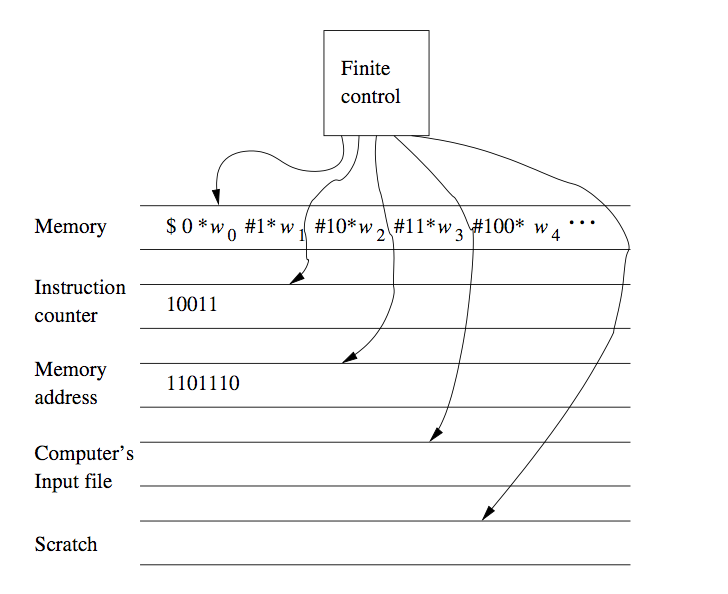
We can prove the latter by using a TM to simulate the instruction cycle of the computer, as follows:
- Search the first tape for an address matching the instruction number on tape 2.
- Examine the instruction address value, if it requires the value of some address, that address is part of the instruction. Mark the position of the instruction using a second tape, not shown in the picture. Search for the memory address on the first tape, an dcopy its value onto tape 3, the tape holding the memory address
- Execute the instruction. Examples of instructions are:
- Copying values to some other address
- Adding value to some other address
- The jump instruction
Runtime of Computers vs Turing Machines
Running time is an important consideration, because we want to know what can be computed with enough efficiency. We divide between tractable and intractable problems, where tractable problems can be solved efficiently.
Hence, we need to assure ourselves that a problem can be solved in polynomial time on a typical computer, can be solved in polynomial time on a TM, and conversely.
A TM can simulate \(n\) steps of a computer in \(O(n^3)\) time. Consider the multiplication instruction: if a computer were to start with a word holding the integer 2, and multiply the word by itself \(n\) times, it would hold the number \(2^{2^n}\), and would take \(2^n + 1\) bits to represent, exponential in \(n\).
To resolve this issue, one can assert that words retain a maximum length. We take another approach, imposing the restriction that instructions may use words of any length, but can only produce words one bit longer than its arguments.
The prove the polynomial time relationship, we note that after \(n\) instructions have been executed, the number of words mentioned on the memory tape of the TM is \(O(n)\), and hence requires \(O(n)\) TM cells to represent. The tape is hence \(O(n^2)\) cells long, and the TM can locate the finite number of words required by one computer instruction in \(O(n^2)\) time.
Hence, if a computer:
- Has only instructions that increase the maximum word length by at most 1, and
- Has only instructions that a multitape TM can perform on wordsd of length \(k\) in \(O(k^2)\) steps or less, then
the Turing machine can simulate \(n\) steps of the computer in \(O(n^3)\) of its own steps.