Compilers
What are compilers?
Compilers are programs that read in one (source) language, and translate them into another (target) language.
Compilers need to perform two main tasks:
- Analysis: breaking up a source program into constituent parts, and create an intermediate representation
- Synthesis: Construct the desired target program from an intermediate representation
A compiler is often designed in a number of phases:
- lexical analyses
- reads a stream of characters, and groups them into a stream of tokens (logically cohesive character sequences). This often requires maintaining a symbol table
- syntax analyses
- imposes a hierarchical structure on the token stream (parse tree)
- semantic analyses
- checks parse tree for semantic errors (e.g. type errors)
- Code optimization
- Optimizes the intermediate code representation in terms of efficiency
- intermediate code generation
- a program for an abstract machine
To contrast this with interpreters, interpreters take as input the program and the data, and produce an output. The interpreters do their computation “online”.
Cousins of the Compiler
- Prepreprocessors
- Macro Processing
- File inclusion
- Language Extension
- Assemblers
- Loaders and Link-editors
The Economy of Programming Languages
Why are there so many programming languages? Application domains have distinctive/conflicting needs. For example, in scientific computing, there needs to be good support for FP, arrays and parallelism. Julia is a good example of a language designed for scientific computing. In systems programming, we require fine control over resources, and satisfy certain real-time constraints. Languages like C are suited for these applications.
Programmer training is the dominant cost for a programming language. It is difficult to modify a language, but easy to start a new one.
Lexical Analyses
The lexical analyzer reads input characters of the source program, group characters into lexemes, and outputs a sequence of tokens to the parser.
It may also:
- Filter out comments and whitespace
- Correlating error messages with source program
- Constructing symbol tables
- Separation of concerns lead to simplicity of design
- Compiler efficiency is improved, when using special techniques
Term Definitions
- token
- <Token name, attribute value>
- pattern
- A description of the formthat can be recognized as a token
- lexeme
- A sequence of characters matching the pattern for a token
E.g. printf("Total = %d", score);
| Tokens | Lexemes |
|---|---|
| id | |
| literal | |
| punctuation |
ID(printf) LBRACE LITERAL("Total = %d") COMMA ID(score) RBRACE SEMI
Tokens have several categories:
| Keywords | if else return |
|---|---|
| Operators | > < <> != ! |
| Identifiers | pi score temp1 |
| Constants | 3.14 “hello” |
| Punctuation | ( ) ; : |
Attributes for tokens distinguish two lexemes belonging to the same symbol table:
<number, 0>, <number, 1>, <price, ptr to symbol table>
Regular Languages
Since the lexical analyzer needs to split splits into token classes, it must be specify the set of strings that belongs into a token class. To do so, we use regular languages.
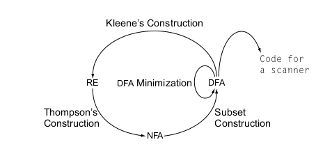
Figure 1: Cycle of constructions
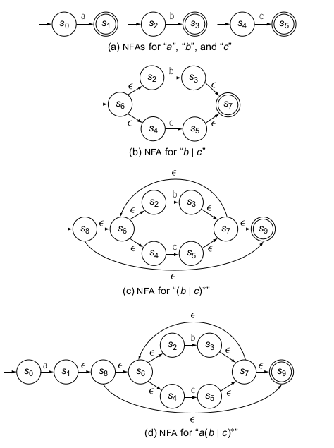
Thompson’s construction
Thompson’s construction converts a regular expression into a NFA. The NFAs derived have several specific properties that simplify an implementation:
- Each NFA has one start state and one end state
- No transition other than the initial transition, enters the start state
- An \(\epsilon\)-transtition always connects two states that were, earlier in the process, the start state and accepting state of NFAs for some component REs
- Each state has at most 2 entering and 2 exiting \(\epsilon\)-moves, and at most one exiting move on a symbol in the alphabet.
Syntax Definition
We use Context-free Grammars to specify the syntax of a language.
A grammar for arithmetic expressions can be constructed from a table showing the associativity and precedence of operators.
  left-associative: + -
  left-associative: * /
Two different non-terminals can be constructed for the two levels of precedence:
  factor -> digit | (expr)
  term -> term * factor
    | term / factor
    | factor
  expr -> expr + term
    | expr - term
    | term
Parsing
Parsers use pushdown automata to do parsing. See LR online parsing machines for an online parsing tool.
Recursive-Descent Parsing
Consists of a set of procedures, one for each non-terminal. The
construction of both top-down and bottom-up parsers is aided by two
functions: first and follow.
\(First(\alpha)\), where \(\alpha\) is any string of grammar symbols, is the set of terminals that begin strings derived from \(\alpha\). If \(\alpha\) derives \(\epsilon\), then \(\epsilon\) is also in \(First(\alpha)\).
Follow(A) for noterminal A, is the set of terminals \(a\) that can appear immediately to the right of A in some sentential form.: the set of terminals \(a\) such that there exists a derivation of the form \(S \overset{**}{\Rightarrow} \alpha A a B\).
Computing First(X)
-
If X is a terminal, then \(First(X) = \{ X \}\)
-
If X is a non-terminal and $X → Y_1 Y_2 … Y_k is a production for some \(k \ge 1\), then place \(a\) in \(First(X)\) for some i, a in \(First(Y_i)\), and ε is in all of \(First(Y_1), \dots, First(Y_{i-1})\). If ε is in \(First(Y_j)\), for all \(j = 1, \dots, k\) then add $ε to \(First(X)\).
-
If \(X \rightarrow \epsilon\) is a production, add \(\epsilon\) to \(First(X)\).
Computing Follow(A)
-
Place $ in \(Follow(S)\), where \(S\) is the start symbol, and $ is the input right endmarker
-
If there is a production \(A \rightarrow \alpha B \beta\) then everything in \(First(\beta)\) except \(\epsilon\) is in \(Follow(B)\).
-
IF there is a production \(A \rightarrow \alpha \beta\), or a production \(A \rightarrow \alpha B \beta\), where \(First(B)\) contains \(\epsilon\), then everything in \(Follow(A)\) is in \(Follow(B)\).
A good video showcasing the computations
LL(1)
A grammar \(G\) is LL(1) if and only if whenever \(A \rightarrow \alpha | \beta\) are two distinct productions of \(G\), the following conditions hold:
- For no terminal $a4 do both \(\alpha\) and \(\beta\) derive strings beginning with \(a\).
- At most one of \(\alpha\) and \(\beta\) can derive the empty string.
- If \(\beta \overset{*}{\Rightarrow} \epsilon\) then $α does n ot derive any string beginning with a terminal in \(Follow(A)\), and vice versa.
Conditions 1 and 2 are equivalent to \(First(\alpha)\) and \(First(\beta)\) being disjoint sets. The third condition is equivalent to stating that if \(\epsilon\) is in \(First(B)\), then \(First(\alpha)\) and \(First(A)\) are disjoint sets, and likewise interchanging \(\alpha\) and \(\beta\).
Bottom-up Parsing
The parse tree for an input string is constructed beginning from the leaves (bottom) and working up towards the root (the top).
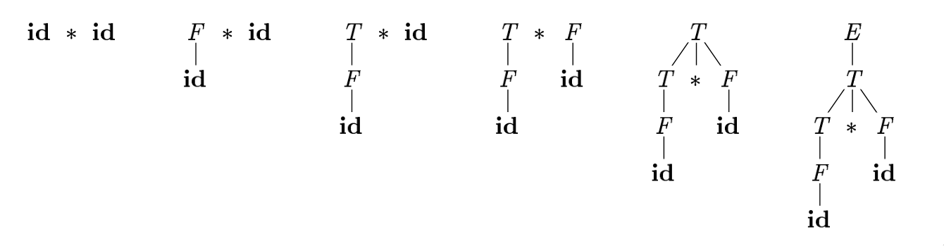
Figure 2: Bottom up parsing
LR grammars can be parsed with shift-reduce parsers.
One can think of bottom-up parsing as the process of “reducing” a string \(w\) to the start symbol of the grammar. At each reduction, a specific substring matching the body of a production is replaced by the nonterminal at the head of the production.
Bottom-up parsing during a left-to-right scan of the input constructs a right-most derivation in reverse.
A stack holds grammar symbols and an inptu buffer holds the rest of the string to be parsed. During a left-to-right scan of the input string, the parser shifts zero or more input symbols onto the stack, until it is ready to reduce a string \(\beta\) of grammar symbols onto the stack. It then reduces \(\beta\) to the head of the appropriate production. The parser repeats this cycle until it has detected an error, or until the stack contains the start symbol and the input is empty.
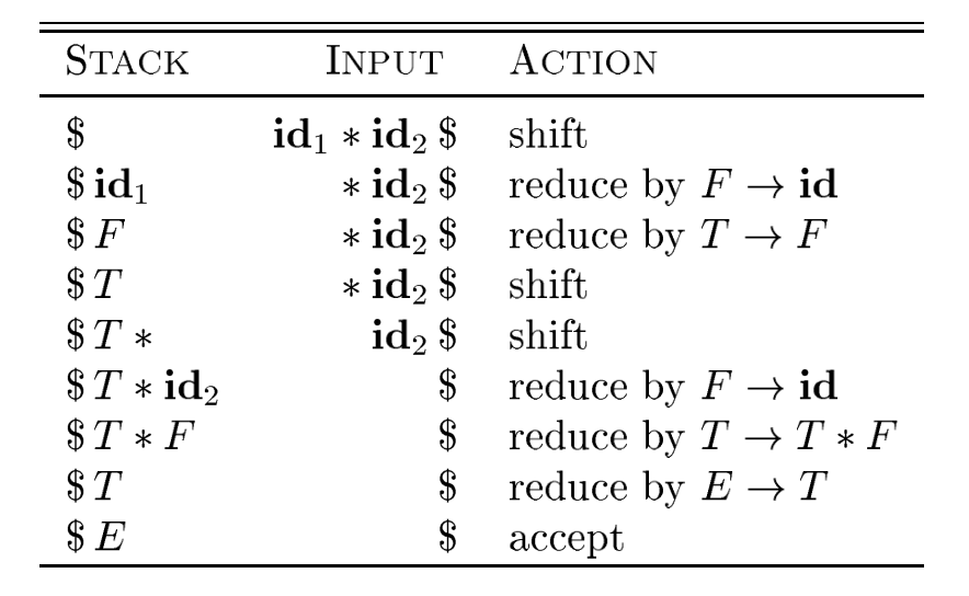
The use of a stack in shift-reduce parsing is because the handle will always eventually appear on top of the stack, and never inside.
Shift-reduce conflicts
- Cannot decide whether to shift or reduce (shift/reduce conflict)
- Cannot decide which of several reductions (reduce/reduce conflict)
These grammars are not in the \(LR(k)\) class of grammars.
In \(LR(k)\), L stands for-to-right scanning, R stands for rightmost derivation. LR parsers are table-driven. The LR-parsing method is the most general nonbacktracking shit-reduce parsing method known. An LR parser can detect a syntactic error as soon as it is possible to do on a left-to-right scan on the input. The class of grammars that can be parsed using LR methods is a proper subset of the class of grammars that can be parsed with predictive or LL methods.
The main downside to this is that construction of a LR parser is tedious by hand.
Syntax Directed Translation
Syntax-directed translation is done by attaching rules or program fragments to productions in a grammar. e.g. consider
expr -> expr_1 + term
We can translate expr by attaching a semantic action within the production body:
expr -> expr_1 + term { print "+" }
The position of the semantic action determines the order in which the action is executed.
The most general approach to SDT is to construct a parse tree or syntax tree, and compute the values of attributes by visiting the nodes of the tree. In most cases, SDT can be performed without explicit construction of the tree.
L-attributed translations (Left to right) encompass all translations that can be performed during parsing.
S-attributed translations (synthesized) is a smaller class that can be performed easily in connection with a bottom-up parse.
Syntax-Directed Definitions
A SDD is a CFG together with attributes and rules. Attributes are associated with grammar symbols, and rules are associated with productions. We write \(X.a\) where \(X\) is a symbol and \(a\) is an attribute.
There are 2 kinds of attributes for non-terminals:
- synthesized attribute
- defined by semantic rule associated with the production at parse tree.
- inherited attribute
- defined by semantic rule associated with the production of parent at parse-tree.
Evaluating an SDD at the nodes of a parse tree
We can construct an annotated parse tree. With synthesized attributes, An SDD with both inherited and synthesized attributes has no guarantee that there is one order in which to evaluate the attributes at nodes. There are useful subclasses of SDDs that are sufficient to guarantee an order of evaluation exists.
The dependency graph characterizes the possible orders in which we can evaluate the attributes at various nodes in the parse tree.
An SDD is S-attributed if every attribute is synthesized. In this scenario, we can evaluate attributes in any bottom-up order, for example using post-order traversal of the parse tree.
In L-attributed SDDs, dependency-graph edges can only go from left-to-right, and not right-to-left. This means that each attribute must be either:
- Synthesized, or
- Inherited, but with rules limited as follows: If there is a
production \( A \rightarrow X_1 X_2 \dots X_n \) and there is an
inherited attribute \(X_i.a\) computed by a rule associated with this
production, then the rule may use only:
- Inherited attributes associated with the head \(A\)
- Either inherited or synthesized attributes associated with the occurrences of symbols \(X_1, X_2 \dots X_{i-1}\) located to the left of \(X_i\).
- Inherited or synthesized attributes associated with \(X_i\) itself, in a way that no cycles are formed in the dependency graph by attributes of this \(X_i\).
Side effecting
We can control side effects in SDDs by:
- Permitting incidental side effects that do not constrain attribute evaluation
- Constrain allowable evaluation orders, so that the translation is produced for any allowable order
Semantic rules executed for their side effects, such as printing, are treade as the definitions of dummy synthesized attributes associated with the head of the production. The modified SDD produces the same translation under any topological sort, since the statement is executed at the end.
Syntax-Directed Translation Schemes
A SDT is a CFG with program fragments embedded within production bodies. The program fragments are called semantic actions, and can appear at any position within the production body.
Run Time Environment
The environment deals out layout and allocation of storage locations in the source program, linkages between procedure and mechanisms for passing parameters, as well as interfaces to the operating system, I/O devices and other programs.
Storage Organization
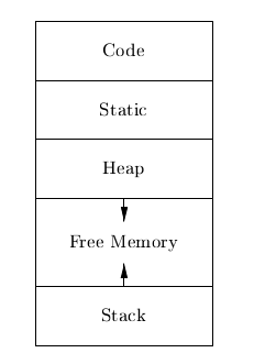
An example of the run-time representation of an object program in the logical address space is shown below:
 The operating system maps logical addresses into physical addresses.
Run-time storage typically comes in blocks of contiguous bytes, where
a byte is the smallest unit of addressable memory.
The operating system maps logical addresses into physical addresses.
Run-time storage typically comes in blocks of contiguous bytes, where
a byte is the smallest unit of addressable memory.
- aligned
- addresses must be divisible by 4
- padding
- space left unused due to alignment issues
The size of a generated target code is fixed at compile time, so the compiler can place the executable target code in a statically determined area called code. The size of program objects like global constants and data is also known at compile time, and is placed at static.
To maximize utilization of space at run-time, the stack and heap are at opposite ends of the remainder of the address space. In practice, the stack grows towards lower addresses, and the heap towards higher, but here we assume the opposite so we can use positive offsets for notational convenience.
Dynamic storage allocation is handled with 2 strategies:
- stack storage
- names local to a procedure are allocated space on the stack
- heap storage
- data that may outlive the call to the procedure are allocated here
Garbage collection enables the run-time system to detect useless data elements and reuse their storage.
Activation Trees
- The sequence of procedure calls corresponds to a preorder traversal of the activation tree
- The sequence of returns corresponds to a postorder traversal of the activation tree
- Suppose that control lies within a particular activation of some procedure, then the activations that are currently open (live) are those that correspond to the node and its ancestors. The order in which these activations are called is the order in which they appear along the path to the node, starting at the root.
Activation Records
Procedure calls and returns are managed by a run-time stack called the control stack. Each live activation has an activation record (frame) on the control stack, with the root of the activation tree at the bottom, and the entire sequence of activation records on the stack corresponding to the path in the activation tree to the activation where control currently resides.
An activation record may contain:
- temporary values
- arising from evaluation of expressions etc.
- local data
- belonging to the procedure whose actiavtion record this is
- saved machine status
- return address (program counter), contents of registers that must be restored when return occurs
- access link
- locate data needed by the called procedure found elsewhere (e.g. in another activation record)
- control link
- pointing to the activation record of the caller
- return value
- space must be allocated for the return value of the called function, if any
- parameters
- Parameters used by the calling procedures, these are however often placed in registers instead of the stack.
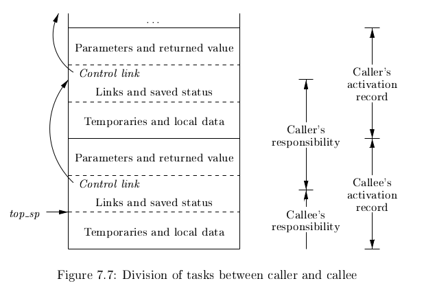
Calling Sequences
Calling sequences consists of code that allocates an activation record on the stack and enters information into its fields. A return sequence similarly contains code that restores the state of the machine so the calling procedure can continue its execution after the call.
It is desirable to put as much of the calling sequence into the callee as possible, but the callee cannot know everything. This reduces the amount of code generated. These are some guiding principles:
- Values communicated between the caller and callee are placed at the beginning of the callee’s activation record, so they are as close as possible to the caller’s activation record. The caller can compute the values of the actual parameters of the call and place them on top of its own activation record without having to create the entire activation record for the callee. It also allows for procedures that have multiple arity.
- Fixed length items are placed in the middle. These include control links, access links and the machine status fields.
- Items whose size may not be known early enough are placed at the end of the activation record. Most local variables have fixed length, which can be determined by the compiler by examining the type of the variable. However, some local variables like dynamically sized arrays cannot be determined until execution.
- We must locate the top-of-stack pointer. A common approach is to have it point to the end of the fixed-length fields in the activation record. Fixed-length data can be accessed by fixed offsets relative to the top-of-stack pointer. The offsets to variable-length fields are then calculated at run-time, using a positive offset from the top-of-stack pointer.
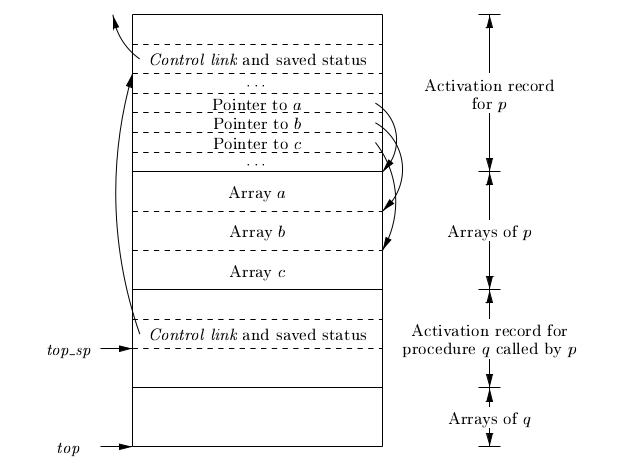
Variable-Length data of the Stack
A common scheme that works for dynamically sized arrays is to have a pointer to the array stored on the stack. This pointer are known offsets from the top-of-stack pointer, so the target code can access array elements through these pointers.
Data Access
Without Nested Procedures
When procedures cannot be nested, allocation of storage for variables is simple:
- Global variables are allocated static storage, the locations are fixed and known at compile time. Access to any variable that is not local to the currently existing procedure can be accessed using the statically determined address.
- Any other name must be local to the activation at the top of the
stack. These variables are accessed through the
top_sppointer of the stack.
This allows declared procedures to be passed as parameters or returned as results (a pointer to the function), without changing the data-access strategy.
With Nested Procedures
Knowing at compile time that the declaration of p is immediately nested in q, says nothing about the relative positions of their activation records at run time.
Finding the declaration that applies to a nonlocal name x in a nested procedure p is a static decision, and can be done by extending the static-scope rule for blocks. The fix for this is to use access links.
If a procedure p is nested immediately within procedure q in the source code, then the access link in any activation of p points to the most recent activation of q. Access links form a chain from the activation record at the top of the stack to a sequence of activations at progressively lower nesting depths.
When procedure q calls procedure p, we consider 2 cases:
- Procedure p is at higher nesting depth than q. If so, then p must be defined immediately within q, or the call by q would not be at a position that is within the scope of prodecure p. Hence, the nesting depth of p is exactly one greater than that of q. In this case the access link for p is a pointer to the activation record of q.
- The nesting depth \(n_p \le n_q\). In order for the call within q to be in the scope of p, q must be nested within some procedure r, while p is a procedure defined within r. The top activation record for r can be found by following the chain of access links, starting in the activation record for q, for \(n_p - n_q + 1\) hops. Then the access link of p must go to activation of r, including recursive calls. The chain of access links is followed for one hop, and the access links for p and q are the same.
When a procedure p is passed to another procedure q as a parameter, then q calls its parameter, it is possible that q does not know the context in which p appears in the program. Hence, the caller needs to pass the proper access link for that parameter.
The caller always knows the link, since if p is passed by procedure r as an actual parameter, then p must be a name accessible to r, and hence r can determine the access link for p as if p were being called by r directly.
Displays
In practice, we use an auxilliary array \(d[i]\) called the display, holding a pointer to the activation records at varying nesting depths \(i\). Since the compiler knows \(i\), it can generate code to access nonlocals with a single access to the display.
To maintain the display properly, we need to save previous values of display entries in the new activation records.
Heap Management
Memory Manager
The memory manager is a subsystem that allocates and deallocates space within the heap.
The desirable properties of a memory manager are:
- space efficiency: minimizing the total heap space required by a program. This allows larger programs to run in a fixed virtual address space.
- program efficiency: make good use of the memory subsystem to allow programs to run faster. This includes exploiting locality.
- low overhead: it should take as little time as possible to allocate and deallocate space. This is however amortized over a large amount of computation.
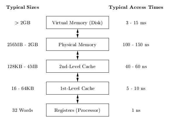
Memory Hierarchy
Locality in programs
- temporal locality
- memory locations it accesses are likely to be accessed again within a short period of time
- spatial locality
- memory access to locations nearby are likely to be accessed within a short period of time
Locality allows us to take advantage of the memory hierarchy, by placing the most common instructions into fast-but-small storage, leaving the rest in slow-but-large storage.
Reducing fragmentation
Free chunks of memory are called holes. With each allocation of memory, the memory manager must place the requested chunk of memory in a large enough hole. Over time, holes will be split into smaller holes for allocation.
Contiguous holes are coalesced into larger holes. However, free memory may end up being fragmented, where a large number of small, non-contiguous holes are available. In this case there is not enough aggregate free space to satisfy a future allocation request.
Best-fit spares the larger holes for future larger requests. First-fit allocates the first hole in which it fits. This takes a smaller amount of time to place objects, but has been found to be inferior to best-fit in overall performance.
To implement best-fit, free space is chunked into bins, according to their sizes. One practical idea is to have many more bins for smaller sizes, because there are usually many more small objects. Larger-
- If there is a bin for chunks of that size only, we may take any chunk from that bin
- For size that do not have a private bin, we find one bin that is allowed to fit chunks of the desired size. Within that bin, we use either a first-fit or best-fit strategy
- If teh target bin is empty, or all chunks in that bin are too small to satisfy the space request, then repeat the search on bins for larger sizes.
Best-fit placement tends to improve space utilization, but often at the expense of spatial locality. One modification is to modify the placement in the case when a chunk of the exact requested size cannot be found. The next-fit strategy tries to allocate the object in the chunk that has last been split, whenever enough space for the new object remains in that chunk.
Coalescing Free Space
When an object is deallocated, we may want to coalesce chunks with adjacent chunks in the heap to form a larger chunk. When we use binning, we may prefer not to do so. Instead, we can simply use a bitmap to indicate whether a chunk is occupied. When a chunk is deallocated, we change the bit from a 1 to 0.
There are 2 data structures that can be used for coalescing chunks when not using binning, or when moving the resultant coalesced chunk into a larger bin.
- Boundary tags: at both the low and high ends of the chunk, we keep a free/used bit that tells us whether or not the block is currently allocated or available. Adjacent to each free/used bit is a count of the total number of bytes in the chunk.
- Doubly-linked, embedded free list: The free chunks are linked in a doubly-linked list. The pointers for this list are within the blocks themselves, e.g. adjacent to the boundary tags at either end. No additional space is required for the free list, although its existence place a lower bound on how small chunks can get: they must accommodate 2 boundary tags and 2 pointers, even if the object is a single byte. The order of chunks on the free list is unspecified: it could be sorted by size to facilitate best-fit placement.
Garbage Collection
There are popular conventions and tools developed to cope with the complexity of managing memory:
- object ownership
- An owner is associated with each object at all times. The owner is a pointer to the object, belonging to some function invocation. The owner is responsible for deleting or passing the object to another owner. Nonowning pointers exist, but cannot delete the object. This eliminates memory leaks, as well as attempts to delete the same object twice. This does not solve the dangling-pointer-reference problem, since it is possible to follow a nonowning pointer to an object that has been deleted. This is useful when an object’s lifetime can be reasoned about statically.
- Reference counting
- A count is associated with each dynamically allocated object. Whenever a reference is removed, the count is decremented. When the count goes to zero, the object can be safely deleted. This does not catch circular data structures. However, it eradicates all dangling-pointer references. This is expensive because it imposes an overhead on every operation that stores a pointer. This is useful when an object’s lifetime needs to be determined dynamically.
- Region-based allocation
- When objects are created to be used only within some step of a computation, we can allocate all such objects in the same region. We then delete the region once the computational step completes. This has limited applicability but is efficient, since the deletion occurs in a wholesale fashion. This is useful when a collection of objects have lifetimes associated with phases of computation.
Garbage collection Design Goals
We assume that objects have types that can be determined at run-time. This allows us to determine the size of the object, and which components of the object contain references to other objects. A user program called the mutator, modifies the collection of objects in the heap. Objects become garbage when the mutator program cannot reach them. The garbage collector finds these unreachable objects and reclaims their space by handing them to the memory manager for deallocation.
Garbage collection can be expensive, so we often want to track performance metrics:
- overall execution time
- space usage
- pause time
- program locality
Reachability
We refer to all data that can be accessed by a program without de-referencing any pointer, as the root set. In Java, this corresponds to all static field members and all variables on its stack.
To find the correct root set, a compiler may have to:
- restrict the invocation of garbage collection to only certain code points in the program
- write out information that the garbage collector can use to recover all the references, such as specifying which registers contain references, or how to compute the base address of an object given its internal address
- the compiler can assure that there is a reference to the base address of all reachable objects whenever the garbage collector is invoked
The set of reachable objects changes as a program executes. There are four basic operations that a mutator performs to change the set:
- Object allocations
- Parameter passing, and return values
- Reference assignments
- Procedure returns
There are 2 approaches to determining reachability:
- Reference counting as an approximation: maintain a count of references to an boject, as the mutator performs actions that may change the set. When the reference count becomes 0, the object is no longer reachable
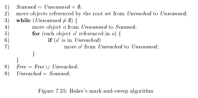
- A trace-based GC labels all objects in the root as reachable, and examines iteratively all references in them to find more reachable objects, and labels them as such. Once the reachable set is computed, it can find many unreachable objects at once. An option is to relocate the reachable objects and reduce fragmentation.
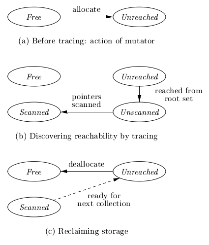
Trace-based GCs
Each chunk is in 1 of 4 states:
- free
- ready to be allocated
- unreached
- chunks presumed to be unreachable, unless proven reachable by tracing. A chunk is in this state at any point during GC if reachability has not yet been established. Whenever a chunk is allocated by the memory manager, its state is set to unreached. After a round of GC, it is reset to unreached for the next round.
- unscanned
- chunks that are known to be reachable are either in state of unscanned or scanned. A chunk is in the unscanned state if it is known to be reachable, but its pointers have not yet been scanned.
- scanned
- every unscanned object will eventually be scanned and transition to the scanned state. To scan an object, we examine all pointers within it, and follow these pointers.
Mark-and-compact GCs
Relocating collectors move reachable objects around in the heap to eliminate memory fragmentation. There are 2 types:
- mark-and-compact, which compacts objects in place. This reduces memory usage.
- copying collector is more efficient, but extra space needs to be reserved for relocation.
mark-and-compact has 3 phases:
- marking phase
- scan the allocated section of the heap and compute new addresses for each of the reachable objects.
- copies objects to the new locations, updating all references in objects that point to the new locations.
Tools
Lex
A Lex compiler takes a Lex source program, and outputs a program. This program is compiled in its source language (originally C, jFlex for Java). The result program takes an input stream as input, and produces a sequence of tokens as output.
A lex program has the following form:
  declarations
  %%
  translation rules
  %%
  auxiliary functions
The declaration section includes declarations of variables, manifest constants, and regular definitions.
The translation rules have form: Pattern { Action }.
Each pattern is a regular expression, which may use the definitions of the declaration section. The actions are fragments of code.
The auxiliary functions section contains used in these actions.