Spiking Neural Networks
Introduction to Spiking Neural Networks
While the project is equal part reinforcement learning and spiking neural networks, reinforcement learning is a popular field and has been extensively covered by researchers worldwide , Ivanov and D’yakonov, n.d., @li18. Hence, I have chosen instead to review the literature around spiking neural networks.
The Generations of Neural Networks
Neural network models can be classified into three generations, according to their computational units: perceptrons, non-linear units, and spiking neurons Maass, n.d..
Perceptrons can be composed to produce a variety of models, including Boltzmann machines and Hopfield networks. Non-linear units are currently the most widely used computational unit, responsible for the explosion of progress in machine learning research, in particular, the success of deep learning. These units traditionally apply differentiable, non-linear activation functions such across a weighted sum of input values.
There are two reasons second-generation computational units have seen so much success. First, the computational power of these units is greater than that of first-generation neural networks. Networks built with second-generation computational units with one hidden layer are universal approximators for any continuous function with a compact domain and range Cybenko, n.d.. Second, networks built with these units are trainable with well-researched gradient-based methods, such as backpropagation.
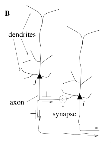
The third generation of neural networks use computational units called spiking neurons. Much like our biological neurons, spiking neurons are connected to each other at synapses, receiving incoming signals at the dendrites and sending spikes to other neurons via the axon. Each computational unit stores some state: in particular, it stores its membrane potential at any point in time. Rather than fire at each propagation cycle, these computational units fire only when their individual membrane potentials crosses its firing threshold. A simple spiking neuron model is given in <spike_model>.
From this section onwards, we shall term second-generation neural networks Artificial Neural Networks (ANNs), and third-generation neural networks Spiking Neural Networks (SNNs).
A Spiking Neuron Model
In spiking neural networks, neurons exchange information via spikes, and the information received depends on:
- Firing frequencies
- The relative timing of pre and post-synaptic spikes, and neuronal firing patterns
- Identity of synapses used
- Which neurons are connected, whether their synapses are inhibitory or excitatory, and synaptic strength
Each neuron has a corresponding model that encapsulates its state: the current membrane potential. As with the mammalian brain, incoming spikes increase the value of membrane potential. The membrane potential eventually decays to resting potential in the absence of spikes. These dynamics are often captured via first-order differential equations. Here we define the Spike Response Model (SRM), a simple but widely-used model describing the momentary value of a neuron \(i\).
We define for presynaptic neuron \(j\), \(\epsilon_{ij}(t) = u_{i}(t) - u_{\text{rest}}\). For a few input spikes, the membrane potential responds roughly linearly to the input spikes:
\begin{equation} u_i{t} = \sum_{j}\sum_{f} \epsilon_{ij}(t - t_j^{(f)}) + u_{\text{rest}} \end{equation}
SRM describes the membrane potential of neuron \(i\) as:
\begin{equation} u_i{t} = \eta (t - \hat{t_i}) + \sum_{j}\sum_{f} \epsilon_{ij}(t - t_j^{(f)}) + u_{\text{rest}} \end{equation}
where \(\hat{t_i}\) is the last firing time of neuron \(i\).
We refer to moment when a given neuron emits an action potential as the firing time of that neuron. We denote the firing times of neuron \(i\) by \(t_i^{(f)}\) where \(f = 1,2,\dots\) is the label of the spike. Then we formally denote the spike train of a neuron \(i\) as the sequence of firing times:
\begin{equation} S_i(t) = \sum_{f} \delta\left( t - t_i^{(f)} \right) \end{equation}
where \(\delta(x)\) is the Dirac-delta function with \(\delta(x) = 0\) for \(x \ne 0\) and \(\int_{-\infty}^{\infty} \delta(x)dx = 1\). Spikes are thus reduced to points in time.
- dendrites
- input device
- soma
- central processing unit (non-linear processing step). If the total input exceeds a certain threshold, an output signal is generated
- axon
- output device, delivering signal to other neurons
- synapse
- junction between two neurons
- post/presynaptic cells
- If a neuron is sending a signal across a synapse, the sending neuron is the presynaptic cell, and the receiving neuron is the postsynaptic cell
- action potentials/spikes
- short electrical pulses, typically of amplitude about 100mV and a duration of 1-2ms
- spike train
- a chain of action potentials (sequence of stereotyped events) that occur at intervals. Since all spikes of a given neuron look the same, the form of the spike does not matter: the number and timing of the spikes encode the information.
- absolute refractory period
- minimal distance between two spikes. Spike are well separated, and it is impossible to excite a second spike within this refractory period.
- relative refractory period
- follows the absolute refractory period – a period where it is difficult to excite an action potential
We define for presynaptic neuron \(j\), \(\epsilon_{ij}(t) = u_{i}(t) - u_{rest}\). For a few input spikes, the membrane potential responds roughly linearly to the input spikes:
\begin{equation} u_i{t} = \sum_{j}\sum_{f} \epsilon_{ij}(t - t_j^{(f)}) + u_{rest} \end{equation}
If \(u_i(t)\) reaches threshold \(\vartheta\) from below, neuron \(i\) fires a spike.
From the above, we can define the Spike Response Model describing the momentary value of the membrane potential of neuron \(i\):
\begin{equation} u_i{t} = \eta (t - \hat{t_i}) + \sum_{j}\sum_{f} \epsilon_{ij}(t - t_j^{(f)}) + u_{rest} \end{equation}
where \(\hat{t_i}\) is the last firing time of neuron \(i\).
We refer to moment when a given neuron emits an action potential as the firing time of that neuron. We denote the firing times of neuron \(i\) by \(t_i^{(f)}\) where \(f = 1,2,\dots\) is the label of the spike. Then we formally denote the spike train of a neuron \(i\) as the sequence of firing times:
\begin{equation} S_i(t) = \sum_{f} \delta\left( t - t_i^{(f)} \right) \end{equation}
where \(\delta(x)\) is the Dirac \(\delta\) function with \(\delta(x) = 0\) for \(x \ne 0\) and \(\int_{-\infty}^{\infty} \delta(x)dx = 1\). Spikes are thus reduced to points in time.
SRM only takes into account the most recent spike, and cannot capture adaptation.
Neuronal Coding
How do spike trains encode information? At present, a definite answer to this question is not known.
Temporal Coding
Traditionally, it had been thought that information was contained in the mean firing rate of a neuron:
\begin{equation} v = \frac{n_{sp}(T)}{T} \end{equation}
measured over some time window \(T\), counting the number of the spikes \(n\). The primary objection to this is that if we need to compute a temporal average to transfer information, then our reaction times would be a lot slower.
From the point of view of rate coding, spikes are a convenient wa of transmitting the analog output variable \(v\) over long spikes. The optimal scheme is to transmit the value of rate \(v\) by a regular spike train at intervals \(\frac{1}{v}\), allowing the rate to be reliably measured after 2 spikes. Therefore, irregularities in real spike trains must be considered as noise.
Rate as spike density (average over several runs)
this definition works for both stationary and time-dependent stimuli. The same stimulation sequence is repeated several times, and the neuronal response is reported in a peri-stimulus-time histogram (PSTH). We can obtain the spike density of the PSTH by:
\begin{equation} \rho(t) = \frac{1}{\Delta t} \frac{n_K(t; t + \Delta t)}{K} \end{equation}
where \(K\) is the number of repetitions of the experiment. We can smooth the results to get a continuous rate.
The problem with this scheme is that it cannot be the decoding scheme of the brain. This measure makes sense if there is always a population of neurons with the same stimulus. This leads to population coding.
Rate as population activity (average over several neurons)
This is a simple extension of the spike density measure, but adding activity across a population of neurons. Population activity varies rapidly and can reflect changes in the stimulus nearly instantaneously, an advantage over temporal coding. However, it requires a homogeneous population of neurons, which is hardly realistic.
Spike Codes
These are coding strategies based on spike timing.
Time-to-first-spike
A neuron which fires shortly after the reference signal (an abrupt input, for example) may signal a strong stimulation, and vice-versa. This estimate has been successfully used in an interpretation of neuronal activity in primate motor cortex.
The argument is that the brain does not have time to evaluate more than one spike per neuron per processing step, and hence the first spike should contain most of the relevant information.
Phase
Oscillations are common in the olfactory system, and other areas of the brain. Neuronal spike trains could then encode information in the phase of a pulse, with respect to the background oscillation.
Correlations and Synchrony
Synchrony between any pairs of neurons could signify special events and convey information not contained in the firing rate of the neurons.
Spikes or Rates?
A code based on time-to-first-spike is consistent with a rate code: if the mean firing rate of a neuron is high, then the time to first spike is expected to occur early. Stimulus reconstruction with a linear kernel can be seen as a special instance of a rate code. It is difficult to draw a clear borderline between pulse and rate codes. The key consideration in using any code is the ability for the system to react quickly to changes in the input. If pulse coding is relevant, information processing in the brain must be based on spiking neuron models. For stationary input, spiking neuron models can be reduced to rate models, but in other cases, this reduction is not possible.
Motivating Spiking Neural Networks
Since second-generation neural networks have excellent performance, why bother with spiking neural networks? In this section, we motivate spiking neural networks from various perspectives.
Information Encoding
To directly compare ANNs and SNNs, one can consider the real-valued outputs of ANNs to be the firing rate of a spiking neuron in steady state. In fact, such rate coding has been used to explain computational processes in the brain Pfeiffer and Pfeil, n.d.. Spiking neuron models encode information beyond the average firing rate: these models also utilize the relative timing between spikes Gütig, n.d., or spike phases (in-phase or out-of-phase). These time-dependent codes are termed temporal codes, and play an important role in biology. First, research has shown that different actions are taken based on single spikes Stemmler, n.d.. Second, relying on the average firing rate would greatly increase the latency of the brain, and our brain often requires decision-making long before several spikes are accumulated. It has also been successfully demonstrated that temporal coding achieves competitive empirical performance on classification tasks for both generated datasets, as well as image datasets like MNIST and CIFAR Comsa et al., n.d..
Biological Plausibility
A faction of the machine learning and neurobiology community strives for emulation of the biological brain. There are several incompatibilities between ANNs and the current state of neurobiology that are not easily reconciliated.
First, neurons in ANNs communicate via continuous-valued activations. This is contrary to neurobiological research, which shows that communication between biological neurons communicate by broadcasting spike trains: trains of action potentials to downstream neurons. The spikes are to a first-order approximation of uniform amplitude, unlike the continuous-valued activations of ANNs.
Second, backpropagation as a learning procedure also presents incompatibilities with the biological brain Tavanaei et al., n.d.. Consider the chain rule in backpropagation:
\begin{equation} \label{chainrule} \delta_{j}^{\mu}=g^{\prime}\left(a_{j}^{\mu}\right) \sum_{k} w_{k j} \delta_{k}^{\mu} \end{equation}
\(\delta_{j}^{\mu}\) and \(\delta_{k}^{\mu}\) denote the partial derivatives of the cost function for input pattern \(\mu\) with respect to the net input to some arbitrary unit \(j\) or \(k\). Unit \(j\) projects feed-forward connections to the set of units indexed by \(k\). \(g(\cdot)\) is the activation function applied to the net input of unit \(j\), denoted \(a_j^{\mu}\), \(w_{kj}\) are the feedforward weights projecting from unit \(j\) to the set of units indexed by \(k\).
The chain rule formulation presents two problems. First, the gradients \(g’(\cdot)\) requires derivatives, but \(g(\cdot)\) in spiking neurons is represented by sum of Dirac delta functions, for which derivatives do not exist. Second, the expression \(\sum_{k} w_{k j} \delta_{k}^{\mu}\) uses feedforward weights in a feedback fashion. This mean that backpropagation is only possible in the presence of symmetric feedback weights, but these do not exist in the brain. In addition, during backpropagation the error assignment for each neuron is computed using non-local information.
Neuromorphic Hardware
In a traditional Von Neumann architecture, the logic core operates on data fetched sequentially from memory. In contrast, in neuromorphic chips both computation and memory are distributed across computational units that are connected via synapses. The neuronal architecture and parameters hence play a key role in information representation and define the computations that are performed.
It has also been observed that spike-trains in the mammalian brain are often sparse in time, suggesting that timing and relative timings of spikes encode large amounts of information. Neuromorphic chips implement this same sparse, low-precision communication protocol between neurons on the chip, and by offering the same asynchronous, event-based parallelism paradigm that the brain uses, are able to perform certain workloads with much less power than Von Neumann chips.
These integrated circuits are typically programmed with spiking neural networks. Examples of such chips include IBM’s TrueNorth Merolla et al., n.d. and Intel’s Loihi Davies et al., n.d.. Because spiking neural networks have not yet been successfully trained on many tasks, neuromorphic chips has seen little practical use. These chips have only recently been successfully used in robotic navigation Tang, Shah, and Michmizos, n.d., and solving graph problems by manual construction of the network graph Severa et al., n.d..
Training Spiking Neural Networks
As explained in
Non-gradient based methods
Spiking neurons communicate via spikes, hence, unlike ANNs, gradients
are non-existent. In addition, backpropagation is not biologically
plausible (see
One category of learning rules used in SNNs are local learning rules. These rules include Hebbian learning (neurons that fire together wire together), and its extension: the spike-timing-dependent-plasticity rule (STDP). Inspired by experiments in neuroscience, central to these learning rules is the theme that neuron spike ordering and their relative timings encode information. STDP adjusts the strength of connections between neurons using the relative timing of a neuron’s output and its input potentials (hence, spike-timing dependent).
In machine learning terminology, the weights of the synapses are adjusted according to fixed rules for each training example. Each synapse is given a weight \(0 \le w \le w_{max}\) , characterizing its strength, and its change depends on the exact moments \(t_{pre}\) of pre-synaptic spikes and \(t_{post}\) of post-synaptic spikes Sboev et al., n.d.:
\begin{equation} \Delta w=\left\{\begin{array}{l}{-\alpha \lambda \cdot \exp \left(-\frac{t_{\mathrm{pre}}-t_{\mathrm{post}}}{\tau_{-}}\right), \text {if } t_{\mathrm{pre}}-t_{\mathrm{post}}>0} \ {\lambda \cdot \exp \left(-\frac{t_{\mathrm{post}}-t_{\mathrm{pre}}}{\tau_{+}}\right), \text {if } t_{\mathrm{pre}}-t_{\mathrm{post}}<0}\end{array}\right. \end{equation}
where \(\tau_{+}\) and \(\tau_{-}\) are time constants. \(\tau_{+} = 16.8ms\) and \(\tau_{-} = 33.7ms\) are reasonable approximations obtained experimentally.
There are several libraries like BindsNET Hazan et al., n.d. that simulate SNNs on Von Neumann computers implementing these rules. Recent attempts have been made to combine Reinforcement Learning and STDP: both in solving RL problems Hazan et al., n.d., and using the reinforcement learning framework to train SNN , Bing et al., n.d., @10.3389/fnins.2018.00435. However, SNNs trained using the STDP learning rule have yet to achieve comparable performance compared to ANNs on relatively simple datasets like MNIST Tavanaei et al., n.d..
Gradient-based methods
Performance is important for practical applications, and gradient-based training methods such as backpropagation has shown competitive performance. It is thus desirable to train spiking neural networks with these gradient-based methods.
There are several problems with spike-compatible gradient-based methods. First, most of these methods cannot train neurons in the hidden layers: they can only train neurons at the final layer, that receive the desired target output pattern Urbanczik and Senn, n.d.. Second, the discontinuous, binary nature of spiking output needs to be addressed. For example, SpikeProp approximates the membrane threshold function at a local area with a linear function, introducing gradients and computing the exact formulae for error backpropagation for synaptic weights and spike times Bohte, Kok, and Poutré, n.d.. Others have modified the threshold function with a gate function NO_ITEM_DATA:huh_gradient_2018, used the alpha transfer function to derive gradient update rules Comsa et al., n.d., and approximate the dirac-delta spikes with a probability density function Shrestha and Orchard, n.d..
Another approach is converting trained ANN models into SNNs Rueckauer et al., n.d.. Common ANN layers such as softmax, batch normalization and max-pooling layers have their corresponding spiking counterparts.
Equilibrium Propagation was recently proposed to solve the neurobiological incompatibilities of backpropagation Scellier and Bengio, n.d.. Because the gradients are defined only in terms of local perturbations, the synaptic updates correspond to the standard form of STDP. The propagated signal encodes the gradients of a well-defined objective function on energy-based models, where the goal is to minimize the energy of the model. To resolve the issue of communication using binary-valued signals, step-size annealing was used to train spiking neural networks with Equilibrium Propagation O’Connor, Gavves, and Welling, n.d..
Future Research Areas
A nascent area is local learning on neuromorphic chips. Thus far spiking neural networks are simulated and trained before deployment on a neuromorphic chip. In Intel’s Loihi chip, each core contains a learning engine that can update synaptic weights using the 4-bit microcode-programmed learning rules that are associated with that synapse. This opens up areas for online learning.
Neural network models can be classified into three generations, according to their computational units: perceptrons, non-linear units, and spiking neurons Maass, n.d..
Perceptrons can be composed to produce a variety of models, including Boltzmann machines and Hopfield networks. Non-linear units are currently the most widely used computational unit, responsible for the explosion of progress in machine learning research, in particular, the success of deep learning. These units traditionally apply differentiable, non-linear activation functions such across a weighted sum of input values.
There are two reasons second-generation computational units have seen so much success. First, the computational power of these units is greater than that of first-generation neural networks. Networks built with second-generation computational units with one hidden layer are universal approximators for any continuous function with a compact domain and range Cybenko, n.d.. Second, networks built with these units are trainable with well-researched gradient-based methods, such as backpropagation.
The third generation of neural networks use computational units called spiking neurons. Much like our biological neurons, spiking neurons are connected to each other at synapses, receiving incoming signals at the dendrites and sending spikes to other neurons via the axon. Each computational unit stores some state: in particular, it stores its membrane potential at any point in time. Rather than fire at each propagation cycle, these computational units fire only when their individual membrane potentials crosses its firing threshold. A simple spiking neuron model is given in <spike_model>.
From this section onwards, we shall term second-generation neural networks Artificial Neural Networks (ANNs), and third-generation neural networks Spiking Neural Networks (SNNs).
A Spiking Neuron Model
In spiking neural networks, neurons exchange information via spikes, and the information received depends on:
- Firing frequencies
- The relative timing of pre and post-synaptic spikes, and neuronal firing patterns
- Identity of synapses used
- Which neurons are connected, whether their synapses are inhibitory or excitatory, and synaptic strength
Each neuron has a corresponding model that encapsulates its state: the current membrane potential. As with the mammalian brain, incoming spikes increase the value of membrane potential. The membrane potential eventually decays to resting potential in the absence of spikes. These dynamics are often captured via first-order differential equations. Here we define the Spike Response Model (SRM), a simple but widely-used model describing the momentary value of a neuron \(i\).
We define for presynaptic neuron \(j\), \(\epsilon_{ij}(t) = u_{i}(t) - u_{\text{rest}}\). For a few input spikes, the membrane potential responds roughly linearly to the input spikes:
\begin{equation} u_i{t} = \sum_{j}\sum_{f} \epsilon_{ij}(t - t_j^{(f)}) + u_{\text{rest}} \end{equation}
SRM describes the membrane potential of neuron \(i\) as:
\begin{equation} u_i{t} = \eta (t - \hat{t_i}) + \sum_{j}\sum_{f} \epsilon_{ij}(t - t_j^{(f)}) + u_{\text{rest}} \end{equation}
where \(\hat{t_i}\) is the last firing time of neuron \(i\).
We refer to moment when a given neuron emits an action potential as the firing time of that neuron. We denote the firing times of neuron \(i\) by \(t_i^{(f)}\) where \(f = 1,2,\dots\) is the label of the spike. Then we formally denote the spike train of a neuron \(i\) as the sequence of firing times:
\begin{equation} S_i(t) = \sum_{f} \delta\left( t - t_i^{(f)} \right) \end{equation}
where \(\delta(x)\) is the Dirac-delta function with \(\delta(x) = 0\) for \(x \ne 0\) and \(\int_{-\infty}^{\infty} \delta(x)dx = 1\). Spikes are thus reduced to points in time.
Motivating Spiking Neural Networks
Since second-generation neural networks have excellent performance, why bother with spiking neural networks? In this section, we motivate spiking neural networks from various perspectives.
Information Encoding
To directly compare ANNs and SNNs, one can consider the real-valued outputs of ANNs to be the firing rate of a spiking neuron in steady state. In fact, such rate coding has been used to explain computational processes in the brain Pfeiffer and Pfeil, n.d.. Spiking neuron models encode information beyond the average firing rate: these models also utilize the relative timing between spikes Gütig, n.d., or spike phases (in-phase or out-of-phase). These time-dependent codes are termed temporal codes, and play an important role in biology. First, research has shown that different actions are taken based on single spikes Stemmler, n.d.. Second, relying on the average firing rate would greatly increase the latency of the brain, and our brain often requires decision-making long before several spikes are accumulated. It has also been successfully demonstrated that temporal coding achieves competitive empirical performance on classification tasks for both generated datasets, as well as image datasets like MNIST and CIFAR Comsa et al., n.d..
Biological Plausibility
A faction of the machine learning and neurobiology community strives for emulation of the biological brain. There are several incompatibilities between ANNs and the current state of neurobiology that are not easily reconciliated.
First, neurons in ANNs communicate via continuous-valued activations. This is contrary to neurobiological research, which shows that communication between biological neurons communicate by broadcasting spike trains: trains of action potentials to downstream neurons. The spikes are to a first-order approximation of uniform amplitude, unlike the continuous-valued activations of ANNs.
Second, backpropagation as a learning procedure also presents incompatibilities with the biological brain Tavanaei et al., n.d.. Consider the chain rule in backpropagation:
\begin{equation} \label{chainrule} \delta_{j}^{\mu}=g^{\prime}\left(a_{j}^{\mu}\right) \sum_{k} w_{k j} \delta_{k}^{\mu} \end{equation}
\(\delta_{j}^{\mu}\) and \(\delta_{k}^{\mu}\) denote the partial derivatives of the cost function for input pattern \(\mu\) with respect to the net input to some arbitrary unit \(j\) or \(k\). Unit \(j\) projects feed-forward connections to the set of units indexed by \(k\). \(g(\cdot)\) is the activation function applied to the net input of unit \(j\), denoted \(a_j^{\mu}\), \(w_{kj}\) are the feedforward weights projecting from unit \(j\) to the set of units indexed by \(k\).
The chain rule formulation presents two problems. First, the gradients \(g’(\cdot)\) requires derivatives, but \(g(\cdot)\) in spiking neurons is represented by sum of Dirac delta functions, for which derivatives do not exist. Second, the expression \(\sum_{k} w_{k j} \delta_{k}^{\mu}\) uses feedforward weights in a feedback fashion. This mean that backpropagation is only possible in the presence of symmetric feedback weights, but these do not exist in the brain. In addition, during backpropagation the error assignment for each neuron is computed using non-local information.
Neuromorphic Hardware
In a traditional Von Neumann architecture, the logic core operates on data fetched sequentially from memory. In contrast, in neuromorphic chips both computation and memory are distributed across computational units that are connected via synapses. The neuronal architecture and parameters hence play a key role in information representation and define the computations that are performed.
It has also been observed that spike-trains in the mammalian brain are often sparse in time, suggesting that timing and relative timings of spikes encode large amounts of information. Neuromorphic chips implement this same sparse, low-precision communication protocol between neurons on the chip, and by offering the same asynchronous, event-based parallelism paradigm that the brain uses, are able to perform certain workloads with much less power than Von Neumann chips.
These integrated circuits are typically programmed with spiking neural networks. Examples of such chips include IBM’s TrueNorth Merolla et al., n.d. and Intel’s Loihi Davies et al., n.d.. Because spiking neural networks have not yet been successfully trained on many tasks, neuromorphic chips has seen little practical use. These chips have only recently been successfully used in robotic navigation Tang, Shah, and Michmizos, n.d., and solving graph problems by manual construction of the network graph Severa et al., n.d..
Training Spiking Neural Networks
As explained in
Non-gradient based methods
Spiking neurons communicate via spikes, hence, unlike ANNs, gradients
are non-existent. In addition, backpropagation is not biologically
plausible (see
One category of learning rules used in SNNs are local learning rules. These rules include Hebbian learning (neurons that fire together wire together), and its extension: the spike-timing-dependent-plasticity rule (STDP). Inspired by experiments in neuroscience, central to these learning rules is the theme that neuron spike ordering and their relative timings encode information. STDP adjusts the strength of connections between neurons using the relative timing of a neuron’s output and its input potentials (hence, spike-timing dependent).
In machine learning terminology, the weights of the synapses are adjusted according to fixed rules for each training example. Each synapse is given a weight \(0 \le w \le w_{max}\) , characterizing its strength, and its change depends on the exact moments \(t_{pre}\) of pre-synaptic spikes and \(t_{post}\) of post-synaptic spikes Sboev et al., n.d.:
\begin{equation} \Delta w=\left\{\begin{array}{l}{-\alpha \lambda \cdot \exp \left(-\frac{t_{\mathrm{pre}}-t_{\mathrm{post}}}{\tau_{-}}\right), \text {if } t_{\mathrm{pre}}-t_{\mathrm{post}}>0} \ {\lambda \cdot \exp \left(-\frac{t_{\mathrm{post}}-t_{\mathrm{pre}}}{\tau_{+}}\right), \text {if } t_{\mathrm{pre}}-t_{\mathrm{post}}<0}\end{array}\right. \end{equation}
where \(\tau_{+}\) and \(\tau_{-}\) are time constants. \(\tau_{+} = 16.8ms\) and \(\tau_{-} = 33.7ms\) are reasonable approximations obtained experimentally.
There are several libraries like BindsNET Hazan et al., n.d. that simulate SNNs on Von Neumann computers implementing these rules. Recent attempts have been made to combine Reinforcement Learning and STDP: both in solving RL problems Hazan et al., n.d., and using the reinforcement learning framework to train SNN , Bing et al., n.d., @10.3389/fnins.2018.00435. However, SNNs trained using the STDP learning rule have yet to achieve comparable performance compared to ANNs on relatively simple datasets like MNIST Tavanaei et al., n.d..
Gradient-based methods
Performance is important for practical applications, and gradient-based training methods such as backpropagation has shown competitive performance. It is thus desirable to train spiking neural networks with these gradient-based methods.
There are several problems with spike-compatible gradient-based methods. First, most of these methods cannot train neurons in the hidden layers: they can only train neurons at the final layer, that receive the desired target output pattern , Urbanczik and Senn, n.d., @10.3389/fnins.2016.00508. Second, the discontinuous, binary nature of spiking output needs to be addressed. For example, SpikeProp approximates the membrane threshold function at a local area with a linear function, introducing gradients and computing the exact formulae for error backpropagation for synaptic weights and spike times Bohte, Kok, and Poutré, n.d.. Others have modified the threshold function with a gate function NO_ITEM_DATA:huh_gradient_2018, used the alpha transfer function to derive gradient update rules Comsa et al., n.d., and approximate the dirac-delta spikes with a probability density function Shrestha and Orchard, n.d..
Another approach is converting trained ANN models into SNNs Rueckauer et al., n.d.. Common ANN layers such as softmax, batch normalization and max-pooling layers have their corresponding spiking counterparts.
Equilibrium Propagation was recently proposed to solve the neurobiological incompatibilities of backpropagation Scellier and Bengio, n.d.. Because the gradients are defined only in terms of local perturbations, the synaptic updates correspond to the standard form of STDP. The propagated signal encodes the gradients of a well-defined objective function on energy-based models, where the goal is to minimize the energy of the model. To resolve the issue of communication using binary-valued signals, step-size annealing was used to train spiking neural networks with Equilibrium Propagation O’Connor, Gavves, and Welling, n.d..
Future Research Areas
A nascent area is local learning on neuromorphic chips. Thus far spiking neural networks are simulated and trained before deployment on a neuromorphic chip. In Intel’s Loihi chip, each core contains a learning engine that can update synaptic weights using the 4-bit microcode-programmed learning rules that are associated with that synapse. This opens up areas for online learning.
Probabilistic SNNs
A probabilistic model defines the outputs of all spiking neurons as jointly distributed binary random processes. The joint distribution is differentiable in the synaptic weights, and principled learning criteria from statistics and information theory such as likelihood and mutual information apply. The maximization of such criteria do not require the implementation of the backpropagation mechanism, and often recover as special cases known biologically plausible algorithms.
Graphical Representation
A SNN consists of a network of \(N\) spiking neurons. At any time \(t = 0,1,2, \dots\) each neouron \(i\) outputs a binary signal \(s_{i,t} = \{0,1\}\), with value \(s_{i,t} = 1\) corresponding to a spike emitted at time \(t\). We collect in vector \(s_{t} = \left( s_{i,t}: i \in V \right)\) the binary signals emitted by all neurons at time \(t\), where \(V\) is the set of all neurons. Each neuron \(i \in V\) receives the signals emitted by a subset \(P_i\) of neurons through directed links, known as synapses. Neurons in a set \(P_i\) are referred to as pre-synaptic for post-synaptic neuron \(i\).
The internal, analog state of each spiking neuron \(i \in V\) at time \(t\) is defined by its membrane potential \(u_{i,t}\).
Long short-term memory and learning-to-learn in networks of spiking neurons Bellec et al., n.d.
Key contribution: Inclusion of adapting neurons into recurrent SNN models (RSNNs) increases computing and learning capability. By using a learning algorithm that combines BPTT with a rewiring algorithm that optimizes the network architecture, performance comes close to LSTM ANNs.
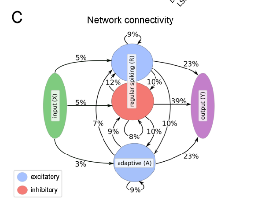
Model composition: LSNNs consist of a populaction \(R\) of integrate-and-fire (LIF) neurons (excitatory and inhibitory), and a second population \(A\) of LIF excitatory neurons whose excitability is temporarily reduced through preceding firing activity. \(R\) and \(A\) receive spike trains from a population \(X\) of external input neurons. Results of computations are read out by a population \(Y\) of external linear readout neurons.
BPTT is done by replacing the non-continuous membrane potential with a pseudo derivative that smoothly increases from 0 to 1.
Learning to Learn LSNNs
LSTM networks are especially suited for L2L since they can accommodate two levelsof learning and representation of learned insight: Synaptic connections and weights can encode,on a higher level, a learning algorithm and prior knowledge on a large time-scale. The short-termmemory of an LSTM network can accumulate, on a lower level of learning, knowledge during thecurrent learning task
Gradient Descent for Spiking Neural Networks
NO_ITEM_DATA:huh_gradient_2018 key idea: Replacing the non-differentiable model for membrane potential:
\begin{equation} \tau \dot{s} = -s + \sum_{k} \delta (t - t_k) \end{equation}
with
\begin{equation} \tau \dot{s} = -s + g \dot{v} \end{equation}
for some gate function \(g\), and \(\dot{v}\) is the time derivative of the pre-synaptic membrane voltage.
Exact gradient calculations can be done with BPTT, or real-time recurrent learning. The resultant gradients are similar to reward-modulated spike-time dependent plasticity.
TODO Surrogate Gradient Learning in Spiking Neural Networks Neftci, Mostafa, and Zenke, n.d.
TODO Theories of Error Back-Propagation in the Brain Whittington and Bogacz, n.d.
Temp Coding with Alpha Synaptic Function
STDP
STDP is a biologically inspired long-term plasticity model, in which each synapse is given a weight \(0 \le w \le w_{maxx}\) , characterizing its strength, and its change depends on the exact moments \(t_{pre}\) of presynaptic spikes and \(t_{post}\) of postsynaptic spikes:
\begin{equation} \Delta w=\left\{\begin{array}{l}{-\alpha \lambda \cdot \exp \left(-\frac{t_{\mathrm{pre}}-t_{\mathrm{post}}}{\tau_{-}}\right), \text {if } t_{\mathrm{pre}}-t_{\mathrm{post}}>0} \ {\lambda \cdot \exp \left(-\frac{t_{\mathrm{post}}-t_{\mathrm{pre}}}{\tau_{+}}\right), \text {if } t_{\mathrm{pre}}-t_{\mathrm{post}}<0}\end{array}\right. \end{equation}
This additive STDP rule requires also an additional constraint that explicitly prevents the weight from falling below 0 or exceeding the maximum value of 1.
Sboev et al., n.d.
Loihi
- Describes SNNs as a weighted, directed graph \( G(V, E)\) where the vertices \(V\) represent compartments, and the weighted edges \(E\) represent synapses.
- Both compartments and synapses maintain internal state and communicate only via discrete spike impulses.
- Uses a variant of the CUBA model for the neuron model, which is defined as a set of first-order differential equation using traces, evaluated at discrete algorithmic time steps.
Learning must follow the sum-of-products form:
\begin{equation} Z(t) = Z(t-1) + \sum_m S_m \prod_n F_n \end{equation}
where \(Z\) is the synaptic state variable defined for the source destination neuron pair being updated, and \(F-N\) may be a synaptic state variable, a pre-synaptic trace or a post-synaptic trace defined for the neuron pair.
Generating Spike Trains
Poisson Model Heeger, n.d.
Independent spike hypothesis: the generation of each spike is independent of all other spikes. If the underlying instantaneous firing rate \(r\) is constant over time, it is a homogeneous Poisson process.
We can write:
\begin{equation} P(\textrm{1 spike during } \delta t) \approx r \delta t \end{equation}
We divide time into short, discrete intervals \(\delta t\). Then, we generate a sequence of random numbers \(x[i]\) uniformly between 0 and 1. For each interval, if \(x[i] \le r \delta t\), generate a spike.