Temp Coding with Alpha Synaptic Function

tags

Spiking Neural Networks

Temporal Coding with Alpha Synaptic Function (Comsa et al., n.d.)

Motivation

1. Atemporal networks (think LSTMs) don’t have the benefits of encoding information directly in the temporal domain
   1. They remain sequential (require all previous layers of computation to produce answer)
   2. Information in the real world are typically temporal

Key Ideas

1. Temporal Coding: Information is encoded in the relative timing of neuron spikes. Using temporal coding allows shift of differentiable relationship into the temporal domain.

   1. Find differentiable relationship of the time of postsynaptic spike with respect to the weights and times of the presynaptic spikes.

2. Alpha synaptic transfer function: Use the SRM, but with the exponential decay of form \(t e^{-t}\).

3. Synchronization pulses: input-independent spikes, used to facilitate transformations of the class boundaries.

The Coding Scheme

More salient information about a feature is encode as an earlier spike in the corresponding input neuron (think time-to-first-spike).

In a classification problem with \(m\) inputs and \(n\) possible classes:

input

spike times of \(m\) input neurons

output

index of output neuron that fires first (among the \(n\) output neurons)

Alpha Synaptic Function

Incoming exponential synaptic kernels are of the form \(\epsilon(t) = \tau^{-1}e^{-\tau t}\) for some decay constant \(\tau\). Potential of membrane in response to the spike is then \(u(t) = t e^{-\tau t}\). It has a gradual rise, and slow decay.

Modelling Membrane Potential

The membrane potential is a weighted sum of the presynaptic inputs:

\begin{equation} V_{mem}(t) = \sum_{i} w_i (t-t_i)e^{\tau(t_i - t)} \end{equation}

We can compute the spike time \(t_{out}\) of a neuron by considering the minimal subset of presynaptic inputs \(I_{t_{out}}\) with \(t_i \le t_{out}\) such that:

\begin{equation} \label{eqn:threshold} \sum_{i \in {I_{t_{out}}}} w_i \left( t_{out} - t_{i} \right) e^{\tau (t_i - t_{out})} = \theta \end{equation}

has 2 solutions: 1 on rising part of function and another on decaying part. The spike time is the earlier solution.

Solving for the Equation

Let \(A_{I} = \sum_{i \in I} w_i e^{\tau t_i}\), and \(B_{I} = \sum_{i \in I} w_i e^{\tau t_i} t_i\), we can compute:

\begin{equation} t_{out} = \frac{B_I}{A_I} - \frac{1}{\tau}W\left( -\tau \frac{\theta}{A_I}e^{\tau \frac{B_I}{A_I}} \right) \end{equation}

where \(W\) is the Lambert W function.

The Loss Function

The loss minimizes the spike time of the target neuron, and maximizes the spike time of non-target neurons (cross-entropy!)

Softmax on the negative values of the spike times \(o_{i}\) (which are always positive):

\begin{equation} p_j = \frac{e^{- o_j}}{\sum_{i=1}^{n} e^{- o_i}} \end{equation}

The cross entropy loss \(L(y_i, p_i) = - \sum_{i=1}^{n} y_i \ln p_i\) is used.

Changing the weights of the network alters the spike times. We can compute the exact derivative of the post synaptic spike time wrt any presynaptic spike time \(t_j\) and its weight \(w_j\) as:

\begin{equation} \frac{\partial t_{out}}{\partial t_j} = \frac{w_j e^{t_j} \left( t_j - \frac{B_I}{A_I} + W_I + 1\right)}{A_I (1 + W_I)} \end{equation}

\begin{equation} \frac{\partial t_{out}}{\partial w_j} = \frac{e^{t_j} \left( t_j - \frac{B_I}{A_I} + W_I + 1\right)}{A_I (1 + W_I)} \end{equation}

where

\begin{equation} W_I = W\left( -\frac{\theta}{A_I}e^{\frac{B_I}{A_I}} \right) \end{equation}

Synchronization Pulses

These act as a temporal form of bias, adjusting class boundaries in the temporal domain. Per network, or per layer biases are added. Spike times for each pulse are learned with the rest of the parameters of the network.

Hyperparameters

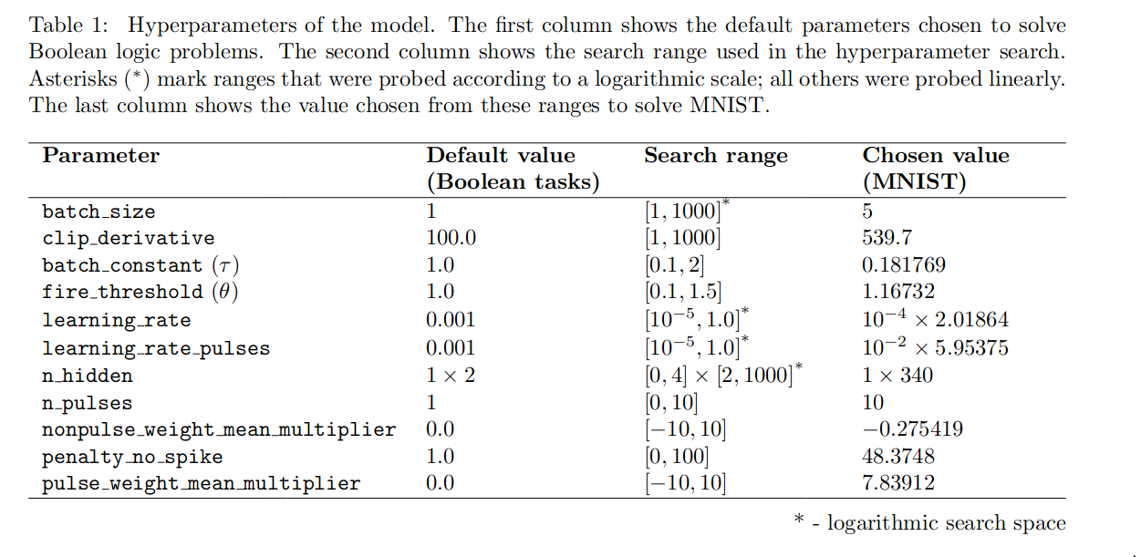
Experiments

Boolean Logic Problems

Inputs encoded as individual spike times of two input neurons. All spikes occur between 0 and 1. True and False values are drawn from distributions \([0.0, 0.45]\) and \([0.55, 1.0]\) respectively.

Trained for maximum of 100 epochs, 1000 training examples. Tested on 150 randomly generated test examples. 100% accuracy on all problems.

Non-convolutional MNIST

784 neurons of the input layer corresponding to pixels of the image. Darker pixels encoded as earlier spike times. Output of network is the index of the earliest neuron to spike.

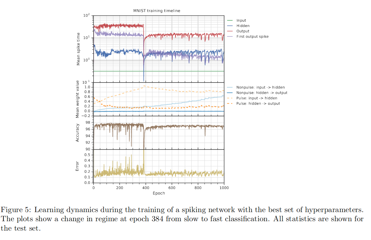
Trained with evolutionary-neural hybrid agents. Best networks achieved 99.96% and 97.96% accuracy on train and test sets.

The network learns two operating modes: slow-regime and fast-regime. Operating in the slow regime has higher accuracy, but takes more time. Fast regime makes quick decisions, with the first spike in the output layer occurring before the mean spike in the hidden layer.

Bibliography

Comsa, Iulia M., Krzysztof Potempa, Luca Versari, Thomas Fischbacher, Andrea Gesmundo, and Jyrki Alakuijala. n.d. “Temporal Coding in Spiking Neural Networks with Alpha Synaptic Function.” http://arxiv.org/abs/1907.13223v1.