Grid & Monte Carlo Localization
Grid & Monte Carlo Localization methods are able to solve global localization problems (in comparison to EKF Localization and Markov Localization).
They also:
- process raw sensor measurements
- are non-parametric: not bound to uni-modal distributions
Grid Localization
The grid localization algorithm uses a histogram filter to represent the posterior belief. Coarseness of the grid is an accuracy, computational-complexity tradeoff. A grid too coarse might prevent the filters from working altogether.
\begin{algorithm} \caption{Grid Localization} \label{grid_localization} \begin{algorithmic}[1] \Procedure{Grid Localization}{$\{p_{k, t-1}\}, u_t, z_t, m$} \ForAll{$k$} \State $\overline{p}_{k,t} = \sum_i p_{i, t-1} \mathbf{\mathrm{motion model}}(\mathrm{mean}(x_k), u_t, \mathrm{mean}(x_i))$ \State $p_{k,t} = \eta \textbf{measurement model}(z_t, \mathrm{mean}(x_k), m)$ \EndFor \State \Return $p_{k,t}$ \EndProcedure \end{algorithmic} \end{algorithm}
Monte-Carlo Localization
MC localization uses the Particle Filter to represent the posterior belief. The accuracy is determined by the size of the particle set.
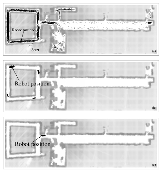
Figure 1: Illustration of MC localization
This algorithm is unable to recover when the pose is incorrect, hence is, without modification, unsuitable for the kidnapped robot problem. This problem is particularly important when the number of particles is small, and when particles are spread over a large volume (with global localization).
This problem can be easily solved by injecting random particles into the particle set. This can be seen as having a small probability of the robot being kidnapped. One can add a fixed number of random particles per iteration, or use an estimate correlated with the localization accuracy, which can be estimated from data.
Another limitation is the proposal mechanism. The particle filter uses the motion model as a proposal distribution, but it seeks to approximate a product of this distribution and the perceptual likelihood. The larger the difference between the proposal and target distribution, the more samples required.
In MCL, this induces a failure mode. A perfect, noiseless sensor would always inform the robot of its correct pose, but MCL would fail. A simple trick that works is to artificially inflate the amount of noise in the sensor. An alternative is to modify the sampling process, by reversing the role of the measurement and motion model for a small number of particles. This results in an algorithm called the mixture MCL.