Computer Vision
Prerequisites
Camera Basics
Single Lens Reflex (SLR)
A camera that typically uses a mirror and prism system that permits the photographer to view through the lens and see exactly what will be captured.
DSLR (Digital SLR)
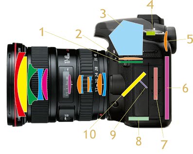
- Matte focusing screen: screen on which the light passing through the lens will project
- Condensing lens: A lens that is used to concentrate the incoming light
- Pentaprism: To produce a correctly oriented, right side up image and project it into the viewfinder eyepiece
- AF sensor: accomplishes auto-focus
- Viewfinder eyepiece: Allows us to see what will be recorded by the image sensor
- LCD Screen: display stored photos or what will be recorded by image sensor
- Image sensor: contains a large number of pixels for converting an optical image into electrical signals. Charge-coupled device (CCD) and Complementary Metal-oxide-semiconductor (CMOS) are the more common ones.
- AE sensor: accomplishes auto exposure
- Sub mirror: To reflect light passing through semi transparent main mirror onto AF sensor
- Main mirror: reflect light into viewfinder compartment. Small semi-transparent area to facilitate AF.
Introduction
Despite the advances in research in computer vision, the dream of having a computer interpret an image at the same level of a human is still far away. Computer vision is inherently a difficult problem, for many reasons. First, it is an inverse problem, in which we seek to recover some unknowns given insufficient information to specify the solution. Hence, we resort to physics-based and probabilistic models to disambiguate between potential solutions.
Forward models that we use in computer vision are usually grounded in physics and computer graphics. Both these fields model how objects move and animate, how light reflects off their surfaces, is scattered by the atmosphere, refracted through camera lenses and finally projected onto a flat image plane.
In computer vision, we want to describe the world that we see in one or more images and to reconstruct its properties, such as shape, illumination and colour distributions. Some examples of computer vision being used in real-world applications include Optical Character Recognition (OCR) , machine inspection, retail, medical imaging, and automotive safety.
In many applications, it is better to think back from the problem at hand to suitable techniques, typical of an engineering approach. A heavy emphasis will be placed on algorithms that are robust to noise, and are reasonably efficient.
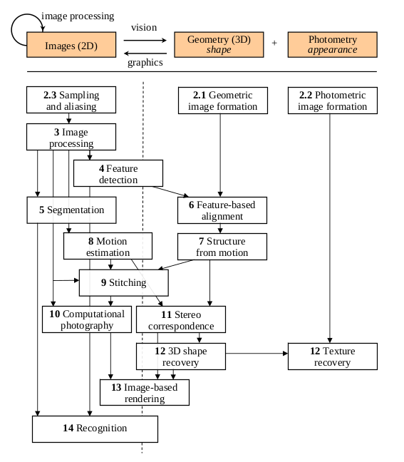
The above figure shows a rough layout of the content of computer vision, and we see that from top to bottom, there are increasing levels of modeling and abstraction.
Image Formation
Geometric Primitives
Geometric primitives form the basic building blocks used to describe three-dimensional shapes.
2D points can be denoted using a pair of values, \(x = (x, y) \in \mathbb{R}^2\):
\begin{equation}
x = \begin{bmatrix}
x \\\
y
\end{bmatrix}
\end{equation}
2D points can also be represented using homogeneous coordinates, \(\tilde{\mathbf{x}} = (\tilde{x}, \tilde{y}, \tilde{w}) \in \mathbb{P}^2\), where vectors that differ only by scale are considered to be equivalent. \(\mathbb{P}^2 = \mathbb{R}^3 - (0, 0, 0)\) is called the 2D projective space.
A homogeneous vector \(\tilde{\mathbf{x}}\) can be converted back into an in-homogeneous vector \(\mathbf{x}\) by diving through the last element \(\tilde{w}\).
2D lines can be represented using homogeneous coordinates \(\tilde{\mathbf{l}} = (a, b, c)\). The corresponding line equation is:
\begin{equation} \bar{\mathbf{x}} \cdot \tilde{\mathbf{l}} = ax + by + c = 0 \end{equation}
The line equation vector can be normalized so that \(\mathbf{l} = (\hat{n}_x, \hat{n}_y, d) = (\hat{\mathbf{n}}, d)\) with \(\lvert \hat{\mathbf{n}} \rvert = 1\). When using homogeneous coordinates, we can compute the intersection of two lines as
\begin{equation} \tilde{\mathbf{x}} = \tilde{\mathbf{l}}_1 \times \tilde{\mathbf{l}}_2 \end{equation}
Similarly, the line joining two points can be written as:
\begin{equation} \tilde{\mathbf{l}} = \tilde{\mathbf{x}}_1 \times \tilde{\mathbf{x}}_2 \end{equation}
Conic sections (which arise from the intersection of a plane and a 3d cone) can be written using a quadric equation
\begin{equation} \tilde{\mathbf{x}}^T\mathbf{Q}\tilde{\mathbf{x}} = 0 \end{equation}
3D points can be written using in-homogeneous coordinates \(\mathbf{x} = (x,y,z) \in \mathbb{R}^3\), or homogeneous coordinates \(\tilde{\mathbf{x}} = (\tilde{x}, \tilde{y}, \tilde{z}, \tilde{w}) \in \mathbb{P}^3\).
3D planes can be represented as homogeneous coordinates \(\tilde{\mathbf{m}} = (a, b, c, d)\) with the equation:
\begin{equation} \bar{\mathbf{x}} \cdot \tilde{\mathbf{m}} = ax + by + cz + d = 0 \end{equation}
3D lines can be represented using 2 points on the line \((\mathbf{p}, \mathbf{q})\). Any other point on the line can be expressed as a linear combination of these 2 points.
\begin{equation} \mathbf{r} = (1 - \lambda)\mathbf{p} + \lambda \mathbf{q} \end{equation}
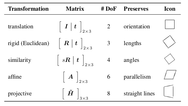
2D Transformations
The basic primitives introduced above can be transformed, the simplest of which occur in the 2D plane.
2D translations can be written as \(\mathbf{x}’ = \mathbf{x} + \mathbf{t}\), or:
\begin{align}
\mathbf{x}’ &= \begin{bmatrix}
\mathbf{I} & \mathbf{t}
\end{bmatrix}\bar{\mathbf{x}} \\\
&= \begin{bmatrix}
\mathbf{I} & \mathbf{t} \\\
\mathbf{0}^T & 1
\end{bmatrix}\bar{\mathbf{x}}
\end{align}
where \(\mathbf{0}\) is the zero vector.
The combination of rotation and translation is known as 2D rigid body motion, or the 2D Euclidean transformation, since Euclidean distances are preserved. It can be written as \(\mathbf{x}’ = \mathbf{R}\mathbf{x} + \mathbf{t}\) or:
\begin{equation} \mathbf{x}’ = \begin{bmatrix} \mathbf{R} & \mathbf{t} \end{bmatrix}\bar{\mathbf{x}} \end{equation}
where
\begin{equation}
\mathbf{R} = \begin{bmatrix}
\cos \theta & - \sin \theta \\\
\sin \theta & \cos \theta
\end{bmatrix}
\end{equation}
is an orthonormal rotation matrix with \(\mathbf{R}\mathbf{R}^T=\mathbf{I}\) and \(\lVert R \rVert = 1\).
The similarity transform, or scaled rotation, can be expressed as \(\mathbf{x}’ = s\mathbf{R}\mathbf{x} + \mathbf{t}\). This preserves angles between lines.
The affine transformation is written as \(\mathbf{x}’ = \mathbf{A}\hat{\mathbf{x}}\), where \(\mathbf{A}\) is an arbitrary \(2 \times 3\) matrix.
Parallel lines remain parallel under affine transformations.
Affine transformations with 6 unknowns can be solved via SVD by forming a matrix equation of the form \(Mx = b\). Local transformations apply different transformations to different regions, and give finer control.
The projective transformation, also known as the perspective transform or homography, operates on homogeneous coordinates:
\begin{equation} \hat{\mathbf{x}}’ = \tilde{\mathbf{H}}\tilde{\mathbf{x}} \end{equation}
where \(\tilde{\mathbf{H}}\) is an arbitrary \(3 \times 3\) matrix. Note that \(\tilde{\mathbf{H}}\) is homogeneous.
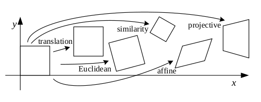
Each of these transformation preserves some properties, and can be presented in a hierarchy.
Some transformations that cannot be classified so easily include:
- Stretching and Squashing
- Planar surface flow
- Bilinear interpolant
The set of 3D transformations are similar to the 2D transformations.
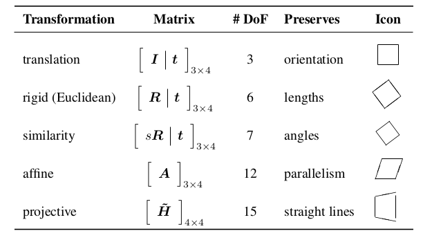
3D Rotations
The biggest difference between 2D and 3D coordinate transformations is that the parameterization of the 3D rotation matrix \(\mathbf{R}\) is not as straightforward.
Euler Angles
A rotation matrix can be formed as the product of three rotations around three cardinal axes, e.g. \(x\), \(y\), and \(z\). This is generally a bad idea, because the result depends on the order of transformations, and it is not always possible to move smoothly in a parameter space.
Axis/angle (exponential twist)
A rotation can be represented by a rotation axis \(\hat{\mathbf{n}}\) and an angle \(\theta\), or equivalently by a 3D vector \(\mathbf{\omega} = \theta\hat{\mathbf{n}}\). We can write the rotation matrix corresponding to a rotation by \(\theta\) around an axis \(\hat{\mathbf{n}}\) as:
\begin{equation} \mathbf{R}(\hat{\mathbf{n}}, \theta) = \mathbf{I} + \sin \theta [\hat{\mathbf{n}}]_\times + \left(1-\cos\theta\right)[\hat{\mathbf{n}}]^2_\times \end{equation}
Also known as Rodriguez’s formula.
For small rotations, this is an excellent choice, as it simplifies to:
\begin{equation}
\mathbf{R}(\mathbf{\omega}) \approx \mathbf{I} + \sin\theta[\hat{\mathbf{n}}]_\times = \begin{bmatrix}
1 & -\omega_x & -\omega_y \\\
\omega_z & 1 & -\omega_x \\\
-\omega_y & \omega_x & 1
\end{bmatrix}
\end{equation}
This gives a nice linearized relationship between the rotation parameters \(\omega\) and \(\mathbf{R}\). We can also compute the derivative of \(\mathbf{R}v\) with respect to \(\omega\),
\begin{equation}
\frac{\partial \mathbf{R}v}{\partial \omega^T} = -[\mathbf{v}]_\times = \begin{bmatrix}
0 & z & -y \\\
-z & 0 & x \\\
y & -x & 0
\end{bmatrix}
\end{equation}
Unit Quarternions
https://eater.net/quaternions https://www.youtube.com/watch?v=d4EgbgTm0Bg
A unit quarternion is a unit length 4-vector whose components can be written as \(\mathbf{q} = (x, y, z, w)\). Unit quarternions live on the unit sphere \(\lVert q \rVert = 1\) and antipodal quartenions, \(q\) and \(-q\) represent the same rotation. This representation is continuous and are very popular representations for pose and for pose interpolation.
Quarternions can be derived from the axis/angle representation through the formula:
\begin{equation} \mathbf{q} = (\mathbf{v}, w) = \left(\sin\frac{\theta}{2}\hat{\mathbf{n}}, \cos\frac{\theta}{2}\right) \end{equation}
where \(\hat{\mathbf{n}}\) and \(\theta\) are the rotation axis and angle. Rodriguez’s formula can be converted to:
\begin{equation} \mathbf{R}(\hat{\mathbf{n}}, \theta) = \mathbf{I} + 2w[\mathbf{v}]_\times + 2[\mathbf{v}]^2_\times \end{equation}
The nicest aspect of unit quarternions is that there is a simple algebra for composing rotations expressed as unit quartenions:
\begin{equation} \mathbf{q}_2 = \mathbf{q}_0 \mathbf{q}_1 = (\mathbf{v}_0 \times \mathbf{v}_1 + w_0 \mathbf{v}_1 + w_1 \mathbf{v}_0, w_0 w_1 - \mathbf{v}_0 \cdot \mathbf{v}_1) \end{equation}
The inverse of a quarternion is just flipping the sign of \(\mathbf{v}\) or \(w\), but not both. Then quarternion division can be defined as:
\begin{equation} \mathbf{q}_2 = \mathbf{q}_0 / \mathbf{q}_1 = (\mathbf{v}_0 \times \mathbf{v}_1 + w_0 \mathbf{v}_1 - w_1 \mathbf{v}_0, - w_0 w_1 - \mathbf{v}_0 \cdot \mathbf{v}_1) \end{equation}
3D to 2D projections
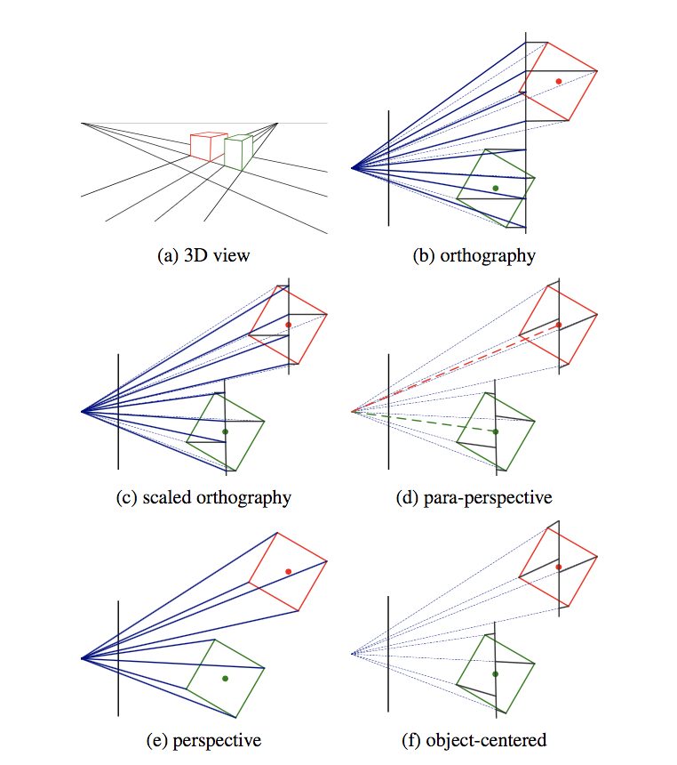
We need to specify how 3D primitives are projected onto the image plane. The simplest model is orthography, which requires no division to get the final (in-homogeneous) result. The more commonly used model is perspective, since this more accurately models the behavior of real cameras.
Orthography
An orthographic projection simply drops the \(z\) component of the three-dimensional coordinate \(\mathbf{p}\) to obtain the 2D point \(\mathbf{x}\).
\begin{equation} \mathbf{x} = \left[\mathbf{I}_{2\times 2} | \mathbf{0} \right] \mathbf{p} \end{equation}
In practice, world coordinates need to be scaled to fit onto an image sensor, for this reason, scaled orthography is actually more commonly used:
\begin{equation} \mathbf{x} = \left[s\mathbf{I}_{2 \times 2}\right | \mathbf{0}]\mathbf{p} \end{equation}
This model is equivalent to first projecting the world points onto a local fronto-parallel image plane, and then scaling this image using regular perspective projection.
A closely related model is called para-perspective, which projects the object points onto a local reference plane parallel to the image plane. However, rather than being projected orthogonally to this plane, they are projected parallel to the line of sight to the object center. This is followed by the usual projection onto the final image plane, and the combination of these two projections is affine.
\begin{equation}
\tilde{\mathbf{x}} = \begin{bmatrix}
a_{00} & a_{01} & a_{02} & a_{03} \\\
a_{10} & a_{11} & a_{12} & a_{13} \\\
0 & 0 & 0 & 1
\end{bmatrix}
\tilde{\mathbf{p}}
\end{equation}
Perspective
Points are projected onto the image plane by dividing them by their \(z\) component. Using homogeneous coordinates, this can be written as:
\begin{equation}
\tilde{\mathbf{x}} = \mathcal{P}_z(\mathbf{p}) = \begin{bmatrix}
x / z \\\
y / z \\\
1
\end{bmatrix}
\end{equation}
In homogeneous coordinates, the projection has a simple linear form,
\begin{equation}
\tilde{\mathbf{x}} = \begin{bmatrix}
1 & 0 & 0 & 0 \\\
0 & 1 & 0 & 0 \\\
0 & 0 & 1 & 0 \\\
\end{bmatrix}\tilde{\mathbf{p}}
\end{equation}
we drop the \(w\) component of \(\mathbf{p}\). Thus after projection, we are unable to recover the distance of the 3D point from the image.
Camera Instrinsics
Once we have projected a 3D point through an ideal pinhole using a projection matrix, we must still transform the resulting coordinates according to the pixel sensor spacing and the relative position of the sensor plane to the origin.
Image sensors return pixel values indexed by integer pixel coordinates \((x_s, y_s)\). To map pixel centers to 3D coordinates, we first scale he \((x_s, y_s)\) values by the pixel spacings \((s_x, s_y)\), and then describe the orientation of the sensor array relative to the camera projection center \(\mathbf{O}_c\) with an origin \(\mathbf{c}_s\) and a 3D rotation \(\mathbf{R}_s\).
\begin{equation}
\mathbf{p} = \left[\mathbf{R}_s | \mathbf{c}_s \right] \begin{bmatrix}
s_x & 0 & 0 \\\
0 & s_y & 0 \\\
0 & 0 & 0 \\\
0 & 0 & 1
\end{bmatrix} \begin{bmatrix}
x_s \\\
y_s \\\
1
\end{bmatrix} = \mathbf{M}_s \hat{\mathbf{x}}_s
\end{equation}
The first 2 columns of the \(3 \times 3\) matrix \(\mathbf{M}_s\) are the 3D vectors corresponding to the unit steps in the image pixel array along the \(x_s\) and \(y_s\) directions, while the third column is the 3D image array origin \(\mathbf{c}_s\).
The matrix \(\mathbf{M}_s\) is parameterized by 8 unknowns, and that makes estimating the camera model impractical, even though there are really only 7 degrees of freedom. Most practitioners assume a general \(3 \times 3\) homogeneous matrix form.
http://ksimek.github.io/2013/08/13/intrinsic/
\begin{align} P &= \overbrace{K}^\text{Intrinsic Matrix} \times \overbrace{[R \mid \mathbf{t}]}^\text{Extrinsic Matrix} \[0.5em] &= \overbrace{
        \underbrace{
            \left (
            \begin{array}{ c c c}
             1  &  0  & x\_0 \\\\\\
             0  &  1  & y\_0 \\\\\\
             0  &  0  & 1
            \end{array}
            \right )
        }\_\text{2D Translation}

        \times

        \underbrace{
            \left (
            \begin{array}{ c c c}
            f\_x &  0  & 0 \\\\\\
             0  & f\_y & 0 \\\\\\
             0  &  0  & 1
            \end{array}
            \right )
        }\_\text{2D Scaling}

        \times

        \underbrace{
            \left (
            \begin{array}{ c c c}
             1  &  s/f\_x  & 0 \\\\\\
             0  &    1    & 0 \\\\\\
             0  &    0    & 1
            \end{array}
            \right )
        }\_\text{2D Shear}

    }^\text{Intrinsic Matrix}

    \times

    \overbrace{
    \underbrace{
         \left( \begin{array}{c | c}
        I & \mathbf{t}
         \end{array}\right)
    }\_\text{3D Translation}
    \times
    \underbrace{
         \left( \begin{array}{c | c}
        R & 0 \\ \hline
        0 & 1
         \end{array}\right)
    }\_\text{3D Rotation}
    }^\text{Extrinsic Matrix}
\end{align}
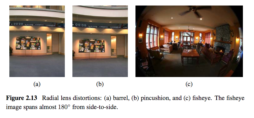
Lens distortion
Thus far, it has been assumed that the cameras obey a linear projection model. In reality, many wide-angled lens suffer heavily from radial distortion, which manifests itself as a visible curvature in the projection of straight lines. Fortunately, compensating for radial distortion is not that difficult in practice. The radial distortion model says that the coordinates in the observed images are displaced away (barrel distortion) or towards (pincushion distortion) the image center by an amount proportional to their radial distance.
Camera Calibration
We want to use the camera to tell us things about the world, so we need the relationship between coordinates in the world, and coordinates in the image.
Geometric camera calibration is composed of:
- extrinsic parameters (camera pose)
- from some arbitrary world coordinate system to the camera’s 3D coordinate system
- intrinsic parameters
- From the 3D coordinates in the camera frame to the 2D image plane via projection
-
Extrinsic Parameters
The transform \(T\) is a transform that goes from the world to the camera system.
-
Translation
The coordinate \(P\) in \(B\)‘s frame is the coordinate \(P\) in frame \(A\), and the location of the camera in frame \(B\).
\begin{equation} ^B P = ^A P + ^B O_A \end{equation}
\begin{equation} \begin{bmatrix} ^B P \\\
1 \end{bmatrix} = \begin{bmatrix} I_{3\times3} & ^B O_A \\\
0^T & 1 \end{bmatrix} \begin{bmatrix} ^A P \\\
1 \end{bmatrix} \end{equation}
-
Rotation
We can similarly describe a rotation matrix:
\begin{equation} ^B P = ^B _A R ^AP \end{equation}
\begin{equation} ^B_A R = \begin{bmatrix} ^B i_A & ^B j_A & ^B k_A \end{bmatrix} = \begin{bmatrix} ^Ai_B^T \\\
^Aj_B^T \\\
^Ak_B^T \end{bmatrix} \end{equation}Under homogeneous coordinates, rotation can also be expressed as a matrix multiplication.
\begin{equation} \begin{bmatrix} ^B P \\\
1 \end{bmatrix} = \begin{bmatrix} ^B_AR & 0 \\\
0^T & 1 \end{bmatrix} \begin{bmatrix} ^A P \\\
1 \end{bmatrix} \end{equation}Then, we can express rigid transformations as:
\begin{equation} \begin{bmatrix} ^B P \\\
1 \end{bmatrix} = \begin{bmatrix} 1 & ^BO_A \\\
0^T & 1 \\\
\end{bmatrix} \begin{bmatrix} ^B_AR & 0 \\\
0^T & 1 \\\
\end{bmatrix} \begin{bmatrix} ^A P \\\
1 \end{bmatrix} = \begin{bmatrix} ^B_AR & ^BO_A \\\
0^T & 1 \end{bmatrix} \begin{bmatrix} ^A P \\\
1 \end{equation}And we write:
\begin{equation} ^B_A T = \begin{bmatrix} ^B_AR & ^BO_A \\\
0^T & 1 \end{bmatrix} \end{equation}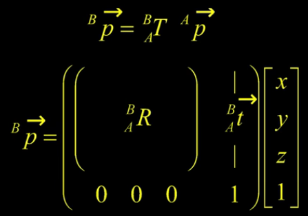
The world to camera transformation matrix is the extrinsic parameter matrix (4x4).
The rotation matrix \(R\) has two important properties:
- \(R\) is orthonormal: \(R^T R = I\)
- \(|R| = 1\)
One can represent rotation using Euler angles:
pitch (\(\omega\)) : rotation about x-axis
yaw (\(\phi\)) : rotation about y-axis
roll (\(\kappa\)) : rotation about z-axis
Euler angles can be converted to rotation matrix:
\begin{align} R &= R_x R_y R_z \end{align}
Rotations can also be specified as a right-handed rotation by an angle \(\theta\) about the axis specified by the unit vector \(\left(\omega_x, \omega_y, \omega_z \right)\).
This has the same disadvantage as the Euler angle representation, where algorithms are not numerically well-conditioned. Hence, the preferred way is to use quarternions. Rotations are represented with unit quarternions.
-
-
Intrinsic Parameters
We have looked at perspective projection, and we obtain the ideal coordinates:
\begin{align} u &= f \frac{X}{Z} \\\
v &= f \frac{Y}{Z} \end{align}However, pixels are arbitrary spatial units, so we introduce an alpha to scale the value.
\begin{align} u &= \alpha \frac{X}{Z} \\\
v &= \alpha \frac{Y}{Z} \end{align}However, pixels may not necessarily be square, so we have to introduce a different parameter for \(u\) and \(v\).
\begin{align} u &= \alpha \frac{X}{Z} \\\
v &= \beta \frac{Y}{Z} \end{align}We don’t know the origin of our camera pixel coordinates, so we have to add offsets:
\begin{align} u &= \alpha \frac{X}{Z} + u_0 \\\
v &= \beta \frac{Y}{Z} + v_0 \end{align}We also assume here that \(u\) and \(v\) are perpendicular. To correct for this, we need to introduce skew coefficients:
\begin{align} u &= \alpha \frac{X}{Z} - \alpha \cot \theta \frac{Y}{Z} + u_0 \\\
v &= \frac{\beta}{\sin \theta} \frac{Y}{Z} + v_0 \end{align}We can simplify this by expressing it in homogeneous coordinates:
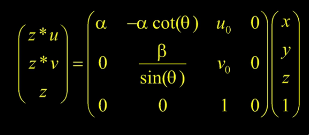
The 3x4 matrix is the intrinsic matrix.
This can be represented in an easier way:
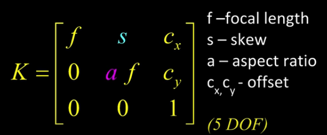
And if we assume:
- pixels are square
- there is no skew
- and the optical center is in the center, then \(K\) reduces to
\begin{equation} K = \begin{bmatrix} f & 0 & 0 \\\
0 & f & 0 \\\
0 & 0 & 1 \end{bmatrix} \end{equation}
-
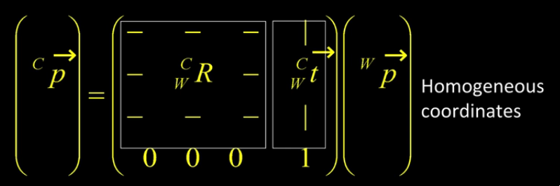
Combining Extrinsic and Intrinsic Calibration Parameters
We can write:
\begin{equation} p’ = K \begin{bmatrix} ^C_WR & ^C_Wt \end{bmatrix} ^Wp \end{equation}
Photometric image formation
Images are not composed of 2D features, but of discrete colour or intensity values. Where do these values come from, and how do they relate to the lighting in the environment, surface properties and geometry, camera optics and sensor properties?
Lighting
To produce an image, a scene must be illuminated with one or more light sources.
A point light source originates at a single location in space. In addition to its location, a point light source has an intensity and a colour spectrum (a distribution over wavelengths).
An area light source with a diffuser can be modeled as a finite rectangular area emitting light equally in all directions. When the distribution is strongly directional, a four-dimensional lightfield can be used instead.
Reflectance and shading
When light hits an object surface, it is scattered and reflected. We look at some more specialized models, including the diffuse, specular and Phong shading models.
-
The Bidirectional Reflectance Distribution Function (BRDF)
Relative to some local coordinate frame on the surface, the BRDF is a four-dimensional function that describes how much of each wavelength arriving at an incident direction \(\hat{\mathbf{v}}_i\) is emitted in a reflected direction \(\hat{\mathbf{v}}_r\). The function can be written in terms of the angles of the incident and reflected directions relative to the surface frame as \(f_r(\theta_i, \phi_i, \theta_r, \phi_r;\lambda)\).
BRDFs for a given surface can be obtained through physical modeling, heuristic modeling or empirical observation. Typical BRDFs can be split into their diffuse and specular components.
-
Diffuse Reflection
The diffuse component scatters light uniformly in all directions and is the phenomenon we most normally associate with shading. Diffuse reflection also often imparts a strong body colour to the light.
When light is scattered uniformly in all directions, the BRDF is constant:
\begin{equation} f_d(\hat{\mathbf{v}}_i, \mathbf{v}}_r, \mathbf{n}};\lambda) = f_d(\lambda) \end{equation}
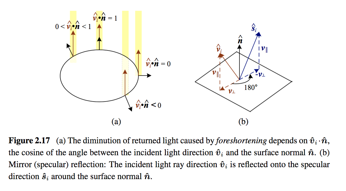
and the amount of light depends on the angle between the incident light direction and the surface normal \(\theta_i\).
-
Specular Reflection
The specular reflection component heavily depends on the direction of the outgoing light. Incident light rays are reflected in a direction that is rotated by 180^° around the surface normal \(\hat{\mathbf{n}}\).
-
Phong Shading
Phong combined the diffuse and specular components of reflection with another term, which he called the ambient illumination. This term accounts for the fact that objects are generally illuminated not only by point light sources but also by a general diffuse illumination corresponding to inter-reflection or distance sources. In the Phong model, the ambient term does not depend on surface orientation, but depends on the colour of both the ambient illumination \(L_a(\lambda)\) and the object \(k_a(\lambda)\),
\begin{equation} f_a(\lambda) = k_a(\lambda) L_a(\lambda) \end{equation}
The Phong shading model can then be fully specified as:
\begin{equation} L_r(\hat{\mathbf{v}}_r ; \lambda) = k_a(\lambda) L_a(\lambda)
- k_d(\lambda) \sum_i L_i(\lambda) [\hat{\mathbf{v}}_i \cdot \hat{\mathbf{n}}]^+
- k_s(\lambda) \sum_i L_i(\lambda) (\hat{\mathbf{v}}_r \cdot \hat{\mathbf{s}}_i)^{k_e} \end{equation}
The Phong model has been superseded by other models in terms of physical accuracy. These models include the di-chromatic reflection model.
-
Optics
Once the light from a scene reaches a camera, it must still pass through the lens before reaching the sensor.
Image Processing
Point Operators
Point operators are image processing transforms where each output pixel’s value depends only on the corresponding input pixel value. Examples of such operators include:
- brightness and contrast adjustments
- colour correction and transformations
Image Enhancement
Histogram Equalization
https://www.math.uci.edu/icamp/courses/math77c/demos/hist%5Feq.pdf
The underlying math behind histogram equalization involves mapping one distribution (the given histogram of intensity values) to another distribution (a wider and, ideally, uniform distribution of intensity values).
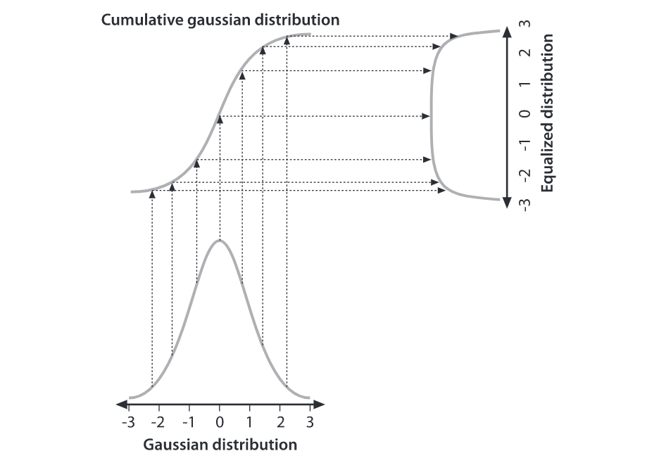
We may use the cumulative distribution function to remap the original distribution as an equally spread distribution simply by looking up each y-value in the original distribution and seeing where it should go in the equalized distribution.
\begin{equation} g_{i,j} = \left\lfloor \left( L - 1 \right) \sum_{n = 0}^{f_{i,j}} p_n \right\rfloor \end{equation}
Convolutions
Convolution is the process of adding each element of the image to its local neighbors, weighted by the kernel.
Convolutions can be used to denoise, descratch, blur, unblur and even feature extraction.
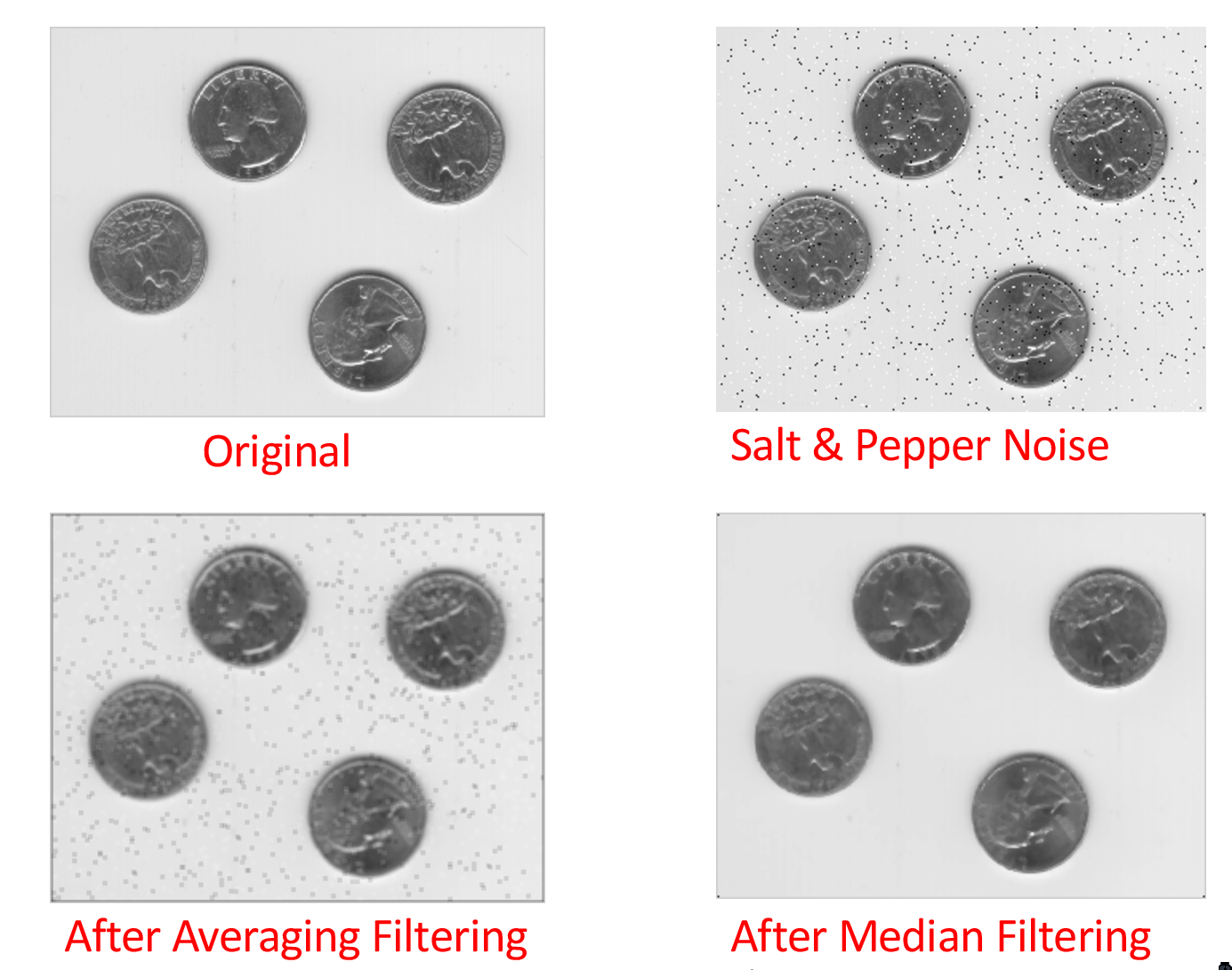
Median filtering is good for removing salt-and-pepper noise, or scratches in image
Color
A human retina has 2 kinds of light receptors: rods are sensitive to amount of light, while cones are sensitive to wavelengths of light
There are 3 kinds of cones:
- short
- most sensitive to blue
- medium
- most sensitive to green
- long
- most sensitive to red
Cones send signals to the brain, and the brain interprets this mixture of signals as colours. This gives rise to the RGB colour coding scheme. Different coding schemes have different colour spaces.
Cones are sensitive to various colours, ranging from wavelengths of 400nm (violet) to 700nm (red).
There are some regions that extend beyond the visible region, but are still relevant to image processing:
- 0.7-1.0\(\mu m\): Near infrared (NIR)
- 1.0-3.0\(\mu m\): Short-wave infrared (SWIR)
- 3.0-5.0\(\mu m\): Mid-wave infrared (MWIR)
- 8.0-12.0\(\mu m\): Long-wave infrared (LWIR)
- 12.0-1000.0\(\mu m\): Far infrared or very long-wave infrared (VLWIR)
The range 5-8\(\mu m\) corresponds to a wavelength spectrum that is largely absorbed by the water in the atmosphere.
Color constancy is the ability of the human visual system to be immune to changing illumination in perception of colour. The human colour receptors perceive the overall effect of the mixture of colours, and cannot tell its composition.
Gamut is the range of colours that can be reproduced with a given colour reproduction system.
In the RGB colour space, each value is an unsigned 8-bit value from 0-255.
In the HSV (Hue Saturation Value) colour space, hue corresponds to colour type from 0 (red) to 360. Saturation corresponds to the colourfulness (0 - 1 full colour), while value refers to the brightness (0 black - 1 white).
The YCbCRr Colour space is used for TV and video. Y stands for luminance, Cb blue difference, and Cr red difference.
There are several colour conversion algorithms to convert values in one colour space to another.
Primary colours are the set of colours combined to make a range of colours. Since human vision is trichromatic, we only need to use 3 primary colours. The combination of primary colours can be additive or subtractive.
Examples of additive combinations include overlapping projected lights and CRT displays. RGB is commonly used in additive combinatinos. Examples of subtracting combinations include mixing of color pigments or dyes. The primary colours used in these cases are normally cyan, magenta and yellow.
Measuring Colour Differences
The simplest metric is the euclidean distance between colours in the RGB space:
\begin{equation} d(C_1, C_2) = \sqrt{\left( R_1 - R_2 \right)^2 + \left( G_1 - G_2 \right)^2 + \left( B_1 - B_2 \right)^2} \end{equation}
However, the RGB space is not perceptually uniform, and this is inappropriate if one needs to match human perception. HSV, YCbCr are also not perceptually uniform. Some colour spaces that are more perceptually uniform are the Munsell, CIELAB and CIELUB colour spaces.
Computing Means
The usual formula of computing means \(M = \frac{1}{n}S = \frac{1}{n}\sum_{i=1}^n R_i\) can lead to overflow even for small \(n\). One way to get around it is to use a floating point representation for \(S\). The second method is to do incremental averaging:
\begin{equation} M_k = \frac{k-1}{k}M_{k-1} + \frac{1}{k}R_k \end{equation}
Digital Cameras sensing colour
Change Detection
Detecting change between 2 video frames is straightforward – compute the differences in pixel intensities across the two frames:
\begin{equation} D_t(x, y) = | I(x,y,t+1) - I(x,y,t)| \end{equation}
It is common to use a threshold for \(D_t(x,y)\) to declare if a pixel has changed.
To detect positional changes, the method used must be immune to illumination change. This requires motion tracking.
At the same time, to detect illumination change, the method must be immune to positional change. In the case of a stationary scene and camera, the straightforward method can be used. However, in the non trivial case, motion tracking will be required.
Motion Tracking
There are two approaches to motion tracking: feature-based and intensity-gradient based.
Feature-based
Feature-based motion tracking utilises distinct features that changes positions. For each feature, we search for the matching feature in the next frame, to check if there is a displacement.
Good features are called “corners”. The two popular corner detectors are the Harris corner detector and the Tomasi corner detector.
Although corners are only a small percentage of the image, they contain the most important features in restoring image information, and they can be used to minimize the amount of processed data for motion tracking, image stitching, building 2D mosaics, stereo vision, image representation and other related computer vision areas.
Harris corner detector
Compared to the Kanade-Lucas-Tomasi corner detector, the Harris corner detector provides good repeatability under changing illumination and rotation, and therefore, it is more often used in stereo matching and image database retrieval.
Interpreting the eigenvalues:
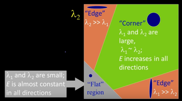
In flat regions, the eigenvalues are both small, in edges, only one of the eigenvalues are large. On the other hand, in corners, both eigenvalues are large but the 2 eigenvalues of the same magnitude, the error \(E\) increases in all directions.
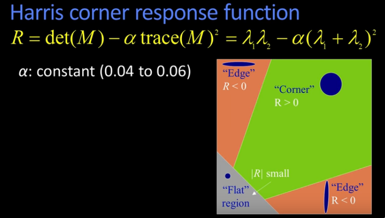
The Harris corner response function essentially filters out the corners.
-
Properties
- Harris corner detector is invariant to rotation: Ellipse has the same eigenvalues regardless of rotation.
- Mostly invariant to additive and multiplicative intensity changes (threshold issue for multiplicative)
- Not invariant to image scale!
Tomasi corner detector
\begin{equation}
\frac{1}{N} \sum_{u} \sum_v \begin{bmatrix}
I_x^2 & I_x I_y \\\
I_x I_y & I_y^2 \\\
\end{bmatrix}
\end{equation}
where \(I_x = \frac{\partial I}{\partial x}\), \(N\) is the total number of pixels in window of interest, \(u\) and \(v\) are the horizontal and vertical index of the pixel in the window of interest.
Let the eigenvalues of the above matrix be \(\lambda_{max}\) and \(\lambda_{min}\). Then the greater \(\lambda_{min}\), the more “cornerness” the feature.
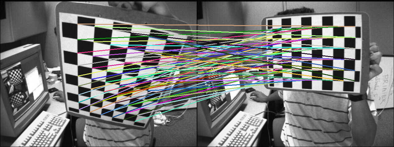
Examples of feature descriptors include SIFT and SURF. The typical workflow involves:
- Detecting good features
- Building feature descriptors on each of these features
- Matching these descriptors on the second image to establish the corresponding points
Gradient-based
Gradient-based motion tracking makes 2 basic assumptions:
- Intensity changes smoothly within image
- Pixel intensities of a given object does not change over time
Suppose that an object is in motion. Then the position of the object is given by \((dx, dy)\) over time \(dt\). From the brightness constancy assumption,
\begin{equation} I(x + dx, y + yd, t + dt) = I(x,y,t) \end{equation}
If we apply the Taylor series expansion on the left hand side, we get:
\begin{equation} I(x + dx, y + dy, t + dt) = I(x,y,t) + \frac{\partial I}{\partial x}dx + \frac{\partial I}{\partial y} dy + \frac{\partial I}{\partial t}dt + \dots \end{equation}
Omitting higher-order terms, we get
\begin{equation} \frac{\partial I}{\partial x}dx + \frac{\partial I}{\partial y} dy + \frac{\partial I}{\partial t}dt = 0 \end{equation}
We denote this as \(I_x u + I_y v + I_t = 0\), but this has 2 unknowns, and is unsolvable.
Lucas-Kanade method
Suppose an object moves by displacement \(\mathbb{d} = (dx, dy)^T\). Then \(J(x+d) = I(x)\), or \(J(x) = I(x-d)\).
Due to noise, there is some error at position \(x\):
\begin{equation} e(x) = I(x - d) - J(x) \end{equation}
We sum the errors over some window \(W\) at position \(x\):
\begin{equation} E(x) = \sum_{x \in W} w(x) \left[ I(x-d) - J(x) \right]^2 \end{equation}
If \(E\) is small, then the patterns in \(I\) and \(J\) match well. We find the \(d\) that minimises \(E\). If we expand \(I(x-d)\) with Taylor expansion:
\begin{equation} I(x-dx, y-dy) = I(x,y) - dx I_x(x,y) - dy I_y (x,y) + \dots \end{equation}
Then,
\begin{equation}
J(x) = I(x - d) = I(x) - d^T g(x), g(x) = \begin{bmatrix}
I_x(x) \\\
I_y(x)
\end{bmatrix}
\end{equation}
Where g(x) is the intensity gradient. Substituting the above equation, and setting \(\frac{\partial E}{\partial d} = 0\):
\begin{equation} \frac{\partial E}{\partial d} = -2 \sum_{x \in W} w(x) \left[ I(x) - J(x) - d^T g(x) \right] g(x) \end{equation}
\begin{equation} \sum_{x \in W} w(x)\left[ I(x) - J(x) \right] g(x) = \sum_{x \in W} w(x) g(x) g^T(x) d \end{equation}
We denote this as:
\begin{equation} Z d = b \end{equation}
where
\begin{equation}
Z = \begin{bmatrix}
\sum_{x \in W} w I_x^2 & \sum_{x \in W} w I_x I_y \\\
\sum_{x \in W} wI_x I_y & \sum_{x \in W} w I_y^2
\end{bmatrix}, b = \begin{bmatrix}
\sum_{x \in W} w(I-J)I_x \\\
\sum_{x \in W} w(I-J)I_y
\end{bmatrix}
\end{equation}
With 2 unknowns and 2 equations, we can solve for \(d\).
Lucas-Kanade algorithm is often used with Harris/Tomasi’s corner detectors. First, corner detectors are applied to detect good features, then LK method is applied to compute \(d\) for each pixel. \(d\) is then accepted only for good features.
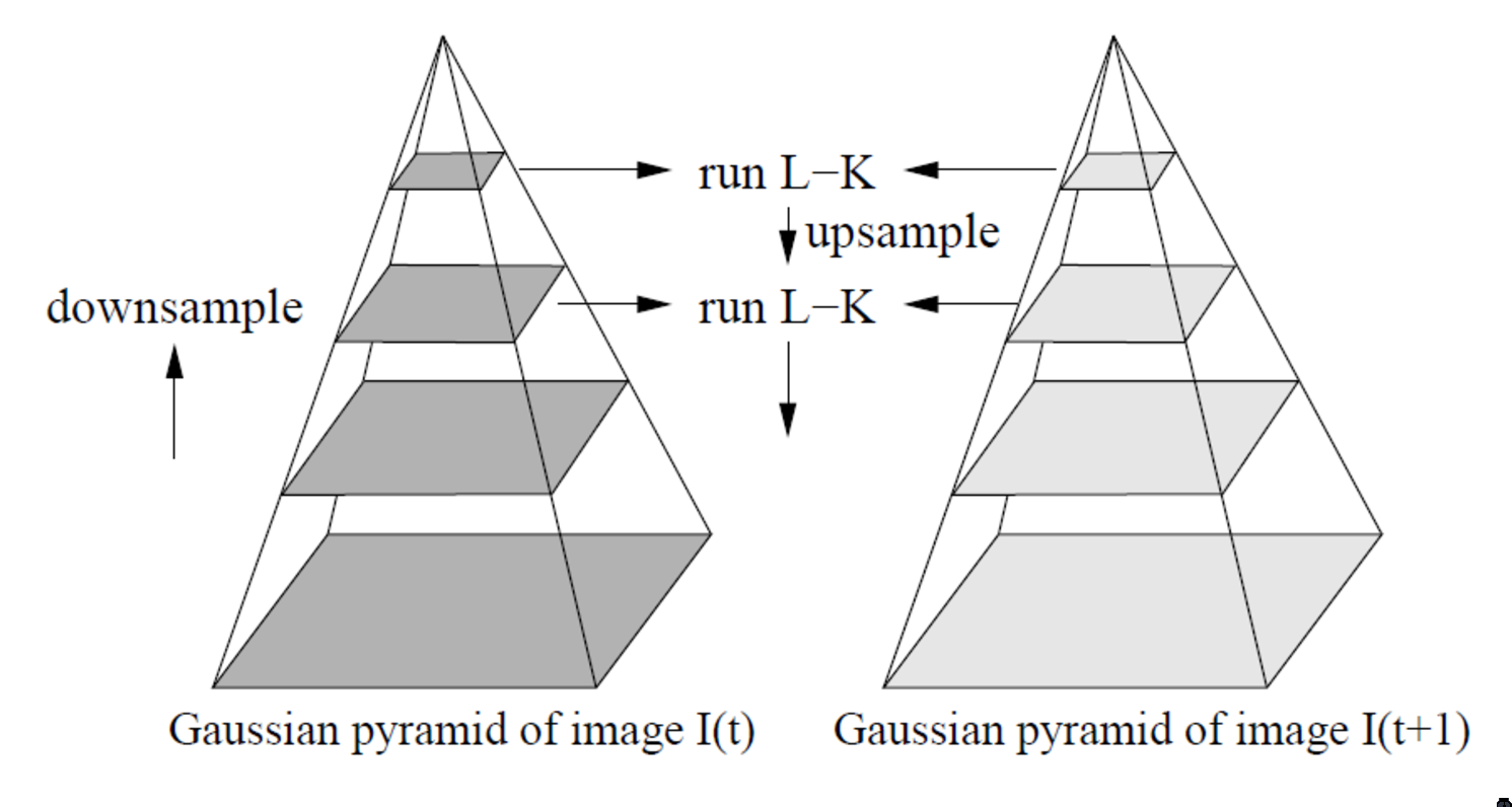
The math of LK tracker assumes \(d\) is small, and would only work for small displacements. To handle large displacements, the image is downsampled. Usually , the Gaussian filter is used to smoothen the image before scaling down.
Homography
https://docs.opencv.org/3.4.1/d9/dab/tutorial%5Fhomography.html
The planar homography relates the transformation between 2 planes, up to a scale factor:
\begin{equation}
s \begin{bmatrix}
x’ \\\
y’ \\\
1
\end{bmatrix} =
H \begin{bmatrix}
x \\\
y \\\
1
\end{bmatrix} =
\begin{bmatrix}
h_{11} & h_{12} & h_{13} \\\
h_{21} & h_{22} & h_{23} \\\
h_{31} & h_{32} & h_{33} \\\
\end{bmatrix}
\begin{bmatrix}
x \\\
y \\\
1
\end{bmatrix}
\end{equation}
The homography is a \(3 \times 3\) matrix with 8 degrees of freedom, as it is estimated up to a scale.
Homographies are used in:
- camera pose estimation
- panorama stitching
- perspective removal/correction
https://cseweb.ucsd.edu/classes/wi07/cse252a/homography%5Festimation/homography%5Festimation.pdf
Structure For Motion
In general, a single image cannot provide 3D information. From a set of images taken with varying camera positions, we can extract 3D information of the scene. This requires us to match (associate) features in one image with the same feature in another image.