Statistical Learning
Introduction
Statistical learning refers to a vast set of tools for understanding data. It involves building a statistical model for predicting, or estimating, an output based on one or more input.
Our goal is to apply a statistical learning method to the training data in order to estimate the unknown function \(f\). Broadly speaking, most statistical learning methods for this task can be characterized as either parametric or non-parametric.
Parametric Methods
Parametric methods involve a two-step model-based approach:
- First, we make an assumption about the functional form, or shape, of \(f\). For example, one simple assumption is that \(f\) is linear in \(X\):
\begin{equation} f(X) = \beta_0 + \beta_1X_1 + \dots + \beta_p X_p \end{equation}
This is a linear model, and with this assumption the problem of estimating \(f\) is greatly simplified. Instead of estimating an arbitrary p-dimensional function \(f(X)\), one only needs to estimate the \(p+1\) coefficients \(\beta_0, \dots, \beta_p\).
After a model has been selected, we need a procedure that uses the training data to fit or train the model. In the case of the linear model, we need to estimate the parameters \(\beta_0, \beta_1, \dots, \beta_p\). The most common approach to fitting the model is referred to as the (ordinary) least squares.
The model-based approach just described is referred to as parametric; it reduces the problem of estimating \(f\) down to one of estimating a set of parameters. The potential disadvantage of a parametric approach is that the model we choose will usually not match the true unknown form of \(f\). If the chosen model is too far from the true \(f\), then our estimate will be poor. Flexible models require a large amount of parameters, and complex models are also susceptible to overfitting.
Non-parametric Methods
Non-parametric methods do not make explicit assumptions about the functional form of \(f\). Instead, they seek an estimate of \(f\) that gets as close to the data points as possible without being too rough or wiggly. By avoiding assumptions of a particular form of \(f\), non-parametric approaches can possibly fit the wider range of possible shapes of \(f\). However, they do not reduce the problem of estimating \(f\) to a small number of parameters, and a large number of observations is required to obtain an accurate estimate for \(f\). An example of a non-parametric model is the thin-plate spline.
The Trade-Off Between Prediction Accuracy and Model Interpretability
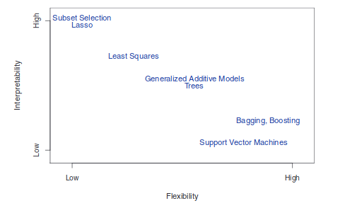
Figure 1: A representation of the tradeoff between flexibility and interpretability, using different statistical methods.
There are several reasons to choose a restrictive model over a flexible approach. First, if the interest is mainly in inference, restrictive models tend to be much more interpretable. For example linear models make it easy to understand the associations between individual predictors and the response. Even when predictions are the only concern, highly flexible models are susceptible to overfitting, and restrictive models can often outperform them.
Measuring Quality of Fit
In order to evaluate the performance of a statistical learning method on a given data set, we need some way to measure how well its predictions actually match the observed data.
In the regression setting, the most commonly-used measure is the mean squared error (MSE), given by:
\begin{equation} \label{eqn:dfn:mse} \mathrm{MSE} = \frac{1}{n} \mathop{\sum}_{i=1}^{n} (y_i - \hat{f}(x_i))^2 \end{equation}
The MSE will be small if the predicted responses are very close to the true responses.
Bias-Variance Trade-Off
It can be shown taht the expected test MSE, for a given value \(x_0\), can always be decomposed into the sum of 3 fundamental qualities: the variance of \(\hat{f}(x_0)\), the squared bias of \(\hat{f}(x_0)\), and the variance of the error terms \(\epsilon\):
\begin{equation} \label{eqn:bvtrade} \mathrm{E} (y_0 - \hat{f}(x_0))^2 = \mathrm{Var}(\hat{f}(x_0)) + \left[ \mathrm{Bias}(\hat{f}(x_0)) \right]^2 + \mathrm{Var}(\epsilon) \end{equation}
The expected test MSE refers to the average test MSE that we would obtain if we repeatedly estimated \(f\) using a large number of training sets, and tested each at \(x_0\).
The variance of a statistical learning method refers to the amount by which \(\hat{f}\) would change if we estimated it using a different training data set. Since the training data are used to fit the statistical learning method, different training data sets will result in a different \(\hat{f}\). In general, more flexible statistical methods have higher variance.
Bias refers to the error that is introduced by approximating a real-life problem, which may be extremely complicated, by a much simpler model. In general, more flexible approaches have lower bias.
The Bayes Classifier
When the test error rate is minimized, the classifier assigns each observation to the most likely class, given its predictor values. This is known as the Bayes classifier. The Bayes classifier produces the lowest possible error rate, known as the Bayes error rate, given by:
\begin{equation} \label{eqn:bayes_error_rate} 1 - \mathrm{E} \left( \mathop{\mathrm{max}}_{j} \mathrm{Pr}(Y = j | X) \right) \end{equation}
In theory, we would always like to predict qualitative responses using the Bayes classifier. However, for real data, we do not know the conditional distribution of \(Y\) given \(X\), and computing the Bayes classifier would be impossible.
K-Nearest Neighbours
The Bayes classifier serves as the unattainable gold standard against which to compare other methods. Many approaches attempt to estimate the conditional distribution of \(Y\) given \(X\), and then classify the given observation to the class with highest estimated probability. One such method is the K-nearest neighbours classifier.
Given a positive integer \(K\) and a test observation \(x_0\), the KNN classifier first identifies the K points in the training data that are closest to \(x_0\), represented by \(N_0\). It then estimates the conditional probability for class \(j\) as the fraction of points in \(N_0\) whose response values equal \(j\):
\begin{equation} \label{eqn:knn} \mathrm{Pr}(Y=j | X = x_0) = \frac{1}{K} \sum_{i\in N_0}I(y_i = j) \end{equation}
Finally, KNN applies Bayes rule and classifies the test observation \(x_0\) to the class with the largest probability.
The Statistical Learning Framework
Consider the problem of classifying a papaya into 2 bins: tasty or not tasty. We’ve chosen 2 features:
- The papaya’s colour, ranging from dark green through orange and red to dark brown
- The papaya’s softness, ranging from rock hard to mushy
The learner’s input consists of:
-
Domain set: An arbitrary set, \(\mathcal{X}\). This is the set of objects that we may wish to label. The domain set in our example will be the set of all papayas. Usually, these domain represented by a vector of features (like colour and softness). We also refer to domain points as instances and to \(\mathcal{X}\) as the instance space.
-
Label set: The label set is restricted in our example to a two-element set, usually {0, 1} or {-1, +1}.
-
Training data: \(S = ((x_1, y_1) \dots (x_m, y_m))\) is a finite sequence of pairs in \(\mathcal{X} \times \mathcal{Y}\). This is the input that the learner has access to. Such labeled examples are often called training examples. \(S\) is also sometimes referred to as the training set.
-
The learner’s output: The learner is requested to output a prediction rule \(h: \mathcal{X} \rightarrow \mathcal{Y}\). This function is also called a predictor, a hypothesis, or a classifier. The predictor can be used to predict the label of new domain points.
-
A simple data-generation model: This explains how the training data is generated. First, we assume that the instances are generated by some probability distribution. We denote the probability distribution over \(\mathcal{X}\) by \(\mathcal{D}\). we do not assume that the learner knows anything about this distribution.
-
Measures of success: We define the error of a classifier to be the probability that it does not predict the correct label on a random data point generated by the underlying distribution. That is, the error of \(h\) is the probability to draw a random instance \(x\) from \(\mathcal{D}\), such that \(h(x) \ne f(x)\), where \(f(x)\) is the true labelling function:
\begin{equation} \label{eqn:dfn:error} L_{\mathcal{D}, f} (h) \overset{\mathrm{def}}{=} \mathop{P}_{x \sim \mathcal{D}} \left[ h(x) \ne f(x) \right] \overset{\mathrm{def}}{=} \mathcal{D} (\{ x: h(x) \ne f(x) \} ) \end{equation}
The learner is blind to the underlying probability distribution \(\mathcal{D}\) over the world, and to the labelling function \(f\). The learner can only interact with the environment through the training set.
Classification
The linear regression model assumes that the response variable \(Y\) is quantitative. However, in many cases the response variable is qualitative. Classification encompasses approaches that predict qualitative responses. 3 of the most widely-used classifiers include: logistic regression, linear discriminant analysis, and K-nearest neighbours. More computer-intensive methods include generalized additive models, trees, random forests, boosting, and support vector machines.
Why not Linear Regression?
Encoding non-binary categorical variables as a dummy variable using integers can lead to a unwanted encoding of a relationship between the different options. With binary outcomes, linear regression does do a good job as a classifier: in fact, it is equivalent to linear discriminant analysis.
Suppose we encode the outcome \(Y\) as follows:
\begin{equation}
Y = \begin{cases}
0 & \text{if No} \\\
1 & \text{if Yes} \\\
\end{cases}
\end{equation}
Then the population \(E(Y|X = x) = \mathrm{Pr}(Y=1|X=x)\), which may seem to imply that regression is perfect for the task. However, linear regression may produce probabilities less than zero or bigger than one, hence logistic regression is more appropriate.
Logistic Regression
Rather than modelling the response \(Y\) directly, logistic regression models the probability that \(Y\) belongs to a particular category.
How should we model the relationship between \(p(X) = \mathrm{Pr}(Y=1|X)\) and \(X\)? In the linear regression model, we used the formula:
\begin{equation} p(X) = \beta_0 + \beta_1 X \end{equation}
This model for \(p(X)\) is not suitable because any time a straight line is fit to a binary response that is coded as a 0 or 1, in principle we can always predict \(p(X) < 0\) for some values of \(X\), and \(p(X) > 1\) for others.
In logistic regression, we use the logistic function:
\begin{equation} p(X) = \frac{e^{\beta_0 + \beta_1 X}}{1 + e^{\beta_0 + \beta_1 X}} \end{equation}
This restricts values of \(p(X)\) to be between 0 and 1. A bit of rearrangement gives:
\begin{equation} \log \left( \frac{p(X)}{1-p(X)} \right) = \beta_0 + \beta_1 X \end{equation}
And this monotone transformation is called the log odds or logit transformation of \(p(X)\).
We use maximum likelihood to estimate the parameters:
\begin{equation} l(\beta_0, \beta) = \prod_{i:y_i=1} p(x_i) \prod_{i:y_i=0} (1 - p(x_i)) \end{equation}
This likelihood gives the probability of the observed zeros and ones in the data. We pick \(\beta_0\) and \(\beta_1\) to maximize the likelihood of the observed data.
As with linear regression, we can compute the coefficient values, the standard error of the coefficients, the z-statistic, and the p-value. The z-statistic plays the same role as the t-statistic. A large absolute value of the z-statistic indicates evidence against the null hypothesis.
Multiple Logistic Regression
It is easy to generalize the formula to multiple logistic regression:
\begin{equation} \log \left( \frac{p(X)}{1-p(X)} \right) = \beta_0 + \beta_1 X_1 + \dots + \beta_p X_p \end{equation}
\begin{equation} p(X) = \frac{e^{\beta_0 + \beta_1X_1 + \dots + \beta_pX_p}}{1 + e^{\beta_0 + \beta_1X_1 + \dots + \beta_pX_p}} \end{equation}
Similarly, we use the maximum likelihood method to estimate the coefficient.
TODO Case Control Sampling
Case control sampling is most effective when the prior probabilities of the classes are very unequal.
Linear Discriminant Analysis
Logistic regression involves directly modelling \(\mathrm{Pr}(Y=k|X=x)\) using the logistic function. We now consider an alternative and less direct approach to estimating these probabilities. We model the distribution of the predictors \(X\) separately in each of the response classes (i.e. given \(Y\)), and then use Bayes’ theorem to flip these around into estimates for \(\mathrm{Pr}(Y=k|X=x)\).
When these distributions are assumed to be normal, it turns out that the model is very similar in form to logistic regression.
Why do we need another method?
- When the classes are well-separated, the parameter estimates for the logistic regression model are surprisingly unstable. LDA does not suffer from this issue.
- If n is small, and the distribution of the predictors \(X\) is approximately normal in each of the classes, the LDA model is more stable than the logistic regression model.
- LDA is more popular when we have more than 2 response classes.
We first state Bayes’ theorem, and write it differently for discriminant analysis:
\begin{equation} {eqn:dfn:bayes} \mathrm{Pr}(Y=k|X=x) = \frac{\mathrm{Pr}(X=x|Y=k) \cdot \mathrm{Pr}(Y=k)}{\mathrm{Pr}(X=x)} \end{equation}
\begin{equation} \mathrm{Pr}(Y=k|X=x) = \frac{\pi_k f_k(x)}{\sum_{l=1}^{K}\pi_lf_l(x)} \end{equation}
where \(f_k(x) = \mathrm{Pr}(X=x|Y=k)\) is the density for \(X\) in class \(k\), and \(\pi_k = \mathrm{Pr}(Y=k)\) is the prior probability for class \(k\).
We first discuss LDA when \(p = 1\). The Gaussian density has the form:
\begin{equation} f_k(x) = \frac{1}{\sqrt{2\pi}\sigma_k}e^{2\frac{1}{2}\left( \frac{x-\mu_k}{\sigma_k} \right)^2} \end{equation}
We can plug this into Bayes formula and get a complicated expression for \(p(x)\). To classify at the value \(X = x\), we just need to see which of \(p_k(x)\) is largest. Taking logs, and discarding terms that do not depend on \(k\), we see that this is equivalent to assigning \(x\) to the class with the largest discriminant score:
\begin{equation} \partial_k(x) = x \cdot \frac{numerator}{\mu_k}{\sigma^2} - \frac{\mu_k^2}{2\sigma^2}+ \log(\pi_k) \end{equation}
Note that \(\partial_k(x)\) is a linear function of \(x\). If there are \(K=2\) classes, and \(\pi_1 = \pi_2 = 0.5\), we can see that the decision boundary becomes \(x = \frac{\mu_1 + \mu_2}{2}\).
We can estimate the parameters:
\begin{equation} \hat{\pi_k} = \frac{n_k}{n} \end{equation}
\begin{equation} \hat{\mu_k} = \frac{1}{n_k}\sum_{i:y_i=k}x_i \end{equation}
\begin{equation} \hat{\sigma}^2 = \frac{1}{n-K}\sum_{k=1}^{K}\sum_{i:y_i=k} (x_i - \hat{\mu_k})^2 \end{equation}
We can extend Linear Discriminant Analysis to the case of multiple predictors. To do that, we will assume that \(X = (X_1, X_2, \dots, X_p)\) is drawn from a multivariate Gaussian distribution, with a class-specific mean vector and a common covariance matrix.
The multivariate Gaussian distribution assumes that each individual predictor follows a one-dimensional normal distribution, with some correlation between each pair of predictors. Formally, the multivariate Gaussian density is defined as:
\begin{equation} f(x) = \frac{1}{(2\pi)^{p/2|\Sigma|^{1/2}}} \mathrm{exp} \left( -\frac{1}{2}(x - \mu)^T \Sigma^{-1}(x - \mu) \right) \end{equation}
In the case of \(p > 1\) predictors, the LDA classifier assumes that the observations in the kith class are drawn from a multivariate Gaussian distribution \(N(\mu_k, \Sigma)\), where \(\Sigma\) is common to all classes. With find that the Bayes classifier assigns an observation \(X = x\) to the class for which:
\begin{equation} \sigma_k(x) = x^T \Sigma^{-1}\mu_k - \frac{1}{2}\mu_k^T\Sigma^{-1}\mu_k + \log \pi_k \end{equation}
The LDA model has the lowest error rate the Gaussian model is correct, since it approximates the Bayes classifier. However, misclassifications can still happen, and a good way to visualize them is through a confusion matrix. The probability threshold can also be tweaked to reduce the error rates for incorrect classification to a single class.
The ROC (Receiver Operating Characteristics) curve is a popular graphic for simultaneously displaying the two types of errors for all possible thresholds. An ideal ROC curve will hug the top left corner, so the larger the AUC (Area Under Curve) the better the classifier. The overall performance of a classifier, summarized over all possible thresholds, is given by this value.
Varying the classifier threshold also changes its true positive and false negative rate. These are also called the sensitivity, and 1 - specificity of the classifier.
Quadratic Discriminant Analysis
In LDA with multiple predictors, we assumed that observations are drawn from a multivariate Gaussian distribution with a class-specific mean vector and a common covariance matrix. Quadratic Discriminant Analysis (QDA) assumes that each class has its own covariance matrix. Under this assumption, the Bayes classifier assigns an observation \(X = x\) to the class for which:
\begin{equation} \partial_k(x) = -\frac{1}{2}(x-\mu_k)^T \Sigma_k^{-1}(x - \mu_k) - \frac{1}{2} \log |\Sigma_k| + \log \pi_k \end{equation}
When would one prefer LDA to QDA, or vice-versa? The answer lies in the bias-variance trade-off. When there are \(p\) predictors, estimating a covariance matrix requires estimating \(p(p+1)/2\) variables. In QDA with \(K\) predictors, we need to estimate \(Kp(p+1)/2\) parameters, which can quickly get big. Hence LDA is much less flexible, and has a lower variance. On the other hand, if the assumption of a common covariance matrix is bad, then LDA will perform poorly.
Comparison of Classification Methods
Logistic Regression and LDA produce linear decision boundaries. The only difference between the two approaches is that in logistic regression the coefficients are estimated using maximum likelihood, while in LDA the coefficients are approximated via the estimated mean and variance from a normal distribution.
Since logistic regression and LDA differ only in their fitting procedures, one might expect the two approaches to give similar results. Logistic regression can outperform LDA if the Gaussian assumptions are not met. On the other hand, LDA can show improvements over logistic regression if they are.
KNN takes a completely different approach from the classifiers seen in this chapter. In order to make a prediction for an observation \(X = x\) , the \(K\) training observations that are closest to \(x\) are identified. Then \(X\) is assigned to the class to which the plurality of these observations belong. Hence KNN is a completely non-parametric approach: no assumptions are made about the shape of the decision boundary. KNN does not tell us which predictors are important, but can outperform LDA and logistic regression if the decision boundary is highly non-linear.
Though not as flexible as the KNN, QDA can perform better in the presence of a limited number of training observations, because it does make some assumptions about the form of the decision boundary.
Reference Textbooks
- An introduction to statistical learning (James et al., n.d.)
- Understanding Machine Learning (Shalev-Shwartz and Ben-David, n.d.)
Bibliography
James, Gareth, Daniela Witten, Trevor Hastie, and Robert Tibshirani. n.d. An Introduction to Statistical Learning. Vol. 112. Springer.
Shalev-Shwartz, Shai, and Shai Ben-David. n.d. Understanding Machine Learning: From Theory to Algorithms. Cambridge university press.