Range Finder Model
Beam Model for Range Finders
4 types of measurement errors are incorporated, all essential to making it work:
- small measurement noise
- errors due to unexpected objects
- errors due to failure to detect objects
- random unexplained noise
The desired model is a mixture of four densities, each of which corresponds to a particular type of error.
Small Measurement Noise
Suppose the true range of the object is \(z_t^{k*}\). The small measurement noise is typically modelled as a narrow Gaussian with mean \(z_t^{k*}\) and standard deviation \(\sigma_{\text{hit}}\). We denote this Gaussian as \(p_{\text{hit}}\).
In practice, the values of the range sensor are limited to the interval \([0; z_{\text{max}}]\), where \(z_{\text{max}}\) denotes the maximum sensor range. Hence, the measurement probability is given by:
\begin{equation} p_{\mathrm{hit}}\left(z_{t}^{k} | x_{t}, m\right)=\left\{\begin{array}{ll}{\eta \mathcal{N}\left(z_{t}^{k} ; z_{t}^{k *}, \sigma_{\mathrm{hit}}^{2}\right)} & {\text { if } 0 \leq z_{t}^{k} \leq z_{\max }} \ {0} & {\text { otherwise }}\end{array}\right. \end{equation}
Unexpected Objects
The environment of mobile robots are dynamics, whereas the map of the environment is static. Examples of moving objects include humans in the environment.
One method of handling these is to include them in the state vector and estimate their position. The simpler way is to treat them as sensor noise. These objects cause ranges to be shorter than \(z_t^{k*}\), not longer.
Since the likelihood of sensing unexpected objects decreases with range, this probability can be described by an exponential distribution, parameterized by \(\lambda_{\text{short}}\).
\begin{equation} p_{\text {short }}\left(z_{t}^{k} | x_{t}, m\right)=\left\{\begin{array}{ll}{\eta \lambda_{\text {short }} e^{-\lambda_{\text {short }} z_{t}^{k}}} & {\text { if } 0 \leq z_{t}^{k} \leq z_{t}^{k *}} \ {0} & {\text { otherwise }}\end{array}\right \end{equation}
Failure to detect objects
This is the situation where objects are missed altogether. This happens often where the object is beyond the sensor’s maximum range. We can model this as a point-mass distribution centered at \(z_{\text{max}}\).
\begin{equation} p_{\max }\left(z_{t}^{k} | x_{t}, m\right)=I\left(z=z_{\max }\right)=\left\{\begin{array}{ll}{1} & {\text { if } z=z_{\max }} \ {0} & {\text { otherwise }}\end{array}\right. \end{equation}
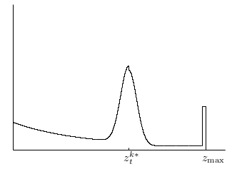
Mixture of the four
The four distributions are mixed by a weighted average:
\begin{equation} p\left(z_{t}^{k} | x_{t}, m\right)=\left(\begin{array}{c}{z_{\text {hit }}} \ {z_{\text {short }}} \ {z_{\text {max }}} \ {z_{\text {rand }}}\end{array}\right)^{T} \cdot\left(\begin{array}{c}{p_{\text {hit }}\left(z_{t}^{k} | x_{t}, m\right)} \ {p_{\text {short }}\left(z_{t}^{k} | x_{t}, m\right)} \ {p_{\text {max }}\left(z_{t}^{k} | x_{t}, m\right)} \ {p_{\text {rand }}\left(z_{t}^{k} | x_{t}, m\right)}\end{array}\right) \end{equation}
Parameters can be learnt from data via maximum likelihood estimation.
Issues
- Can be unsmooth in the presence of many small obstacles: this poses a problem for ML estimation
- Computationally expensive