Neural Ordinary Differential Equations
Motivation
In this section, I motivate the benefits of Neural Ordinary Differential Equations (ODEs). Many physical phenomena can be modeled naturally with the language of differential equations. These include populations of predator and prey, or in physics with regard to motion between bodies. Differential equations shine where it is easier to model changes in the systems over time rather than the value themselves.
Consider a simple pendulum, with the dampening effect of air resistance. One can model the dynamic system using a second-order ODE, as such:
\begin{equation} \ddot{\theta}(t) = - \mu \dot{\theta}(t) - \frac{g}{L}\sin\left( \theta(t) \right) \end{equation}
There are infinitely many solutions to this ODE, but generally only one that satisfies the initial conditions at \(t = 0\). We’d like to find \(\theta(t)\) for some any \(t\). It turns out finding the solutions to these problems are hard, and numerical methods are required to find the solutions. These numerical methods range from simplest Euler’s method, to Runge-Kutta methods.
Suppose now that we have some dynamic system (for example, the pendulum), and we have measured some data from the system \(\hat{\theta}(t)\) (the pendulum’s position, at time \(t\)). Can a neural network learn the dynamics of the system from data?
Regular neural networks states are transformed by a series of discrete transformations:
\begin{equation} \mathbf{h}_{t+1} = f(\mathbf{h}_t) \end{equation}
where \(f\) could be of different kinds of layers, including convolutional and dense layers. \(t\) can be interpreted as a time index, transforming some input data at \(t=0\) to an output in a different space at \(t=N\), where there are \(N\) layers.
Because neural networks apply discrete transformations, to learn dynamical systems with (recurrent) neural networks, one must discretize the time steps, for example through binning the observations into fixed time intervals. However, expressing time as a discrete variable can be unnatural: this includes processes where events occur at irregular intervals. This means that the current state-of-the-art neural networks are still unable to model continuous sequential data.
The Analogy to Residual Neural Networks
In neural networks, every layer introduces error that compounds through the neural network, hindering overall performance. The only way to bypass this is to add more layers, and limit the complexity of each step. This means that the highest performing neural networks would have infinite layers, and infinitesimal step-changes, an infeasible task.
To address this problem, deep residual neural networks were presented He et al., n.d.; Dupont, Doucet, and Teh, n.d..
Instead of learning \(h_{t+1} = f(h_t, \theta_t)\), deep residual neural networks now learn the difference between the layers: \(h_{t+1} = h_t + f(h_t, \theta_t)\). For example, feed-forward residual neural networks have a composition that looks like these:
\begin{align*}
h_1 &= h_0 + f(h_0, \theta_0) \\\
h_2 &= h_1 + f(h_1, \theta_1) \\\
h_3 &= h_2 + f(h_2, \theta_2) \\\
\dots \\\
h_{t+1} &= h_t + f(h_t, \theta_t) \\\
\end{align*}
These iterative updates correspond to the infinitesimal step-changes described earlier, and can be seen to be analogous to an Euler discretization of a continuous transformation Lu et al., n.d.. In the limit, one can instead represent the continuous dynamics between the hidden units using an ordinary differential equation (ODE) specified by some neural network:
\begin{equation} \frac{d\mathbf{h}(t)}{dt} = f(\mathbf{h}(t), t, \theta) \end{equation}
where the neural network has parameters \(\theta\). The equivalent of having \(T\) layers in the network, is finding the solution to this ODE at time \(T\).
The analogy between ODEs and neural networks is not new, and has been discussed in previous papers , Haber and Ruthotto, n.d., @lu17. This paper popularized this idea, by proposing a new method for scalable backpropagation through ODE solvers, allowing end-to-end training within larger models.
The NeuralODE Model
The Neural ODE model introduces a new type of block the authors term the ODE block. This block replaces the ResNet-like skip connections, with an ODE that models the neural network’s dynamics:
\begin{equation} \frac{d\mathbf{h}(t)}{dt} = f(\mathbf{h}(t), t, \theta) \end{equation}
This ODE can then be solved using a black box solver, with the output state being used to compute the loss:
\begin{equation} L(\mathbf{z}(t_1)) = L\left( \mathbf{z}(t_0) + \int_{t_0}^{t_1} f(\mathbf{z}(t), t, \theta)dt \right) = L(\textrm{ODESolve}(\mathbf{z}(t_0), f, t_0, t_1, \theta)) \end{equation}
The loss is used to compute gradients, but, as mentioned in the paper, performing backpropagation through the ODE solver incurs too high a memory cost. Here, I illustrate why, with a simple example.
Suppose we use the Euler method to solve the ODE. The Euler solver update step is similar to a ResNet block:
\begin{equation} h_{t+1} = h_t + NN(h_{t}) \end{equation}
Continuous-depth networks will have large \(t\). Despite the ODE solvers being easily differentiable, backpropagating through the neural network in this case is equivalent to computing and storing the gradients in a $t$-depth ResNet. With higher-order ODE solvers, the memory requirements are also higher.
The paper proposes a method of computing gradients by solving a second, augmented ODE backwards in time, that is applicable to all ODE solvers.
Gradient Computation via Adjoint Sensitivity Analysis
If one wishes to train a Neural ODE via gradient descent, one would need to compute gradients for the loss function \(L(\textrm{ODESolve}(\mathbf{z}(t_0), f, t_0, t_1, \theta))\). This requires propagation of gradients through the ODE-solver, that is, gradients with respect to \(\theta\). The paper proposes a technique that scales linearly with problem size, has low memory cost, and explicitly controls numerical error.
Sensitivity analysis defines a new ODE whose solution gives the gradients to the cost function w.r.t. the parameters, and solves this secondary ODE. Because the gradients of the loss is dependent on the hidden state \(z(t)\) at each instant, the dynamics of \(z(t)\) can be represented with yet another ODE. Obtaining the gradients would require a single solve by recomputing \(z(t)\) backwards together with the adjoint. The derivations are provided in the appendix of the paper, and will not be repeated here. Chen et al., n.d.
Since a large part of the paper’s contribution is the ability to bridge many years of mathematical advancements on solving differential equations, it is wise to analyse the pros and cons of other solvers in the context of training machine learning models.
Traditional adjoint sensitivity analysis require multiple forward solutions of the ODE, which can become prohibitively costly in large models. The paper’s proposal reduces the computational complexity to a single solve, while retaining low memory cost by solving the backwards solution together with the adjoint. One issue that the paper has failed to address is that their proposed method requires that the ODE integrator is time-reversible. There are no ODE solvers for first-order ODEs that are time-reversible, implying that the method proposed will diverge on some systems rackauckas19_diffeq.
In general, while the model is agnostic of the choice of ODE solver, the ideal choice of differential equation solver depends on the problem to be solved. For different classes of differential equations (under certain assumptions), some solvers will prove to be more efficient or more accurate. A good rule of thumb is that forward-mode automatic differentiation is efficient for differential equations with a small number of parameters, while reverse-mode automatic differentiation is more efficient when the model size grows bigger.
Replacing ResNets
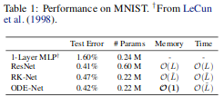
Because an ODE block is simply the continuous version of the Residual block, it seems plausible to use ODE blocks as replacements for ResNet blocks. The authors of the paper experimented with MNIST, and found that using ODE blocks they were able to achieve roughly equivalent test-error, with a third of the parameters (0.22M compared to 0.60M) and constant memory cost during training.
While this looks promising, it would be more instructive to train the ODEnet on different datasets.
It turns out that because of the continuous limit, there is a class of functions that Neural ODEs. In particular, Neural ODEs can only learn features that are homeomorphic to the input space Dupont, Doucet, and Teh, n.d.. The errors arising from discretization allow ResNet trajectories to cross, allowing them to represent certain flows that Neural ODEs cannot.
Experiments
To understand Neural ODEs, I referenced several implementations. First, I ran the implementation provided with the paper. With the provided code, it was easy to reproduce the results of the Neural ODE model for MNIST.
To further understand the how to write solvers for ODEs and the Adjoint method, I referenced the implementations from a seminar. The example notebooks provided were small and self-contained, I wrote the naive ODE solver using Euler’s method, and swapped out the adjoint ODE solver. Even for a relatively dataset of relatively small dimensionality, using it to train on the MNIST dataset took an hour. Each epoch took slightly longer than the previous, which the authors attribute to the increasing number of function evaluations, as a result of the model adapting to increasing complexity. Perhaps one could place a penalty on model complexity (something like MDL), to prevent overfitting, and maintain interpretability of the learnt model.
In general, I found that the gains from having to train a model with fewer parameters is offset by the difficulty in training. In my experiments conducted, the full data-set is passed for evaluation and gradient descent is used to update the parameters. The authors have mentioned that mini-batching, and using stochastic gradient descent is tricky. Doing a full gradient descent may be infeasible where the dataset is too large, and the sub-gradients cannot fit into memory.
ODE as Prior Knowledge
A use-case that I have not seen discussed with the introduction of Neural ODEs is the ability to introduce structure to the machine learning models.
Suppose we have collected data from some known dynamic system, and wish to learn the system. Traditional machine learning models have no way of specifying the structure of the dynamic system, and the model would have to learn its model parameters solely from the data. However, supposing we know the equations governing the dynamic system: for example, it is a system for which the laws of physics govern the system (gravitational attraction between objects). We can then restrict the hypothesis class to the family of functions that satisfy the equations, while ensuring that learning is still realizable (there exists the correct hypothesis \(h^*\) in the subclass \(\mathcal{H’}\)). Restricting the hypothesis space would lead to lower sample complexity.
Closing Thoughts
This paper presented a new family of models called Neural ODEs. They naturally arise by taking the continuous limit in residual neural networks. The paper proposes a numerically unstable, but empirically working method for performing back-propagation through black-box ODE solvers, making training neural ODEs feasible.
While not novel, this paper brought into the limelight the idea of marrying differential equations with machine-learning, an area that has seemingly a lot of potential.
From experimentation, I find that Neural ODEs are still difficult to train beyond simple problems, and mathematical theory shows that the choice of the ODE solver is still important.
In this review, I did not cover the applications of Neural ODEs in other areas. First, they have a particularly convenient formulation for Continuous Normalizing Flows. Normalizing flows is a technique for sampling from complex distributions via sampling from a simple distribution, and has applications in techniques like variational inference.
EDIT: During NeurIPS 2019, David Duvenaud reflects on the claims and the hype of the Neural ODE paper.
Bibliography
[rackauckas19_diffeq] Rackauckas, Innes, Ma, Bettencourt, White & Dixit, Diffeqflux.Jl - a Julia Library for Neural Differential Equations, CoRR, . link. ↩