Machine Teaching

Definitions Simard et al., n.d.

machine learning research

machine learning research aims at making the learner better by improving ML algorithms

machine teaching research

machine teaching research aims at making the teacher more productive at building machine learning models

Problem Formulation

Machine learning takes a given training dataset \(D\) and learns a model \(\hat{\theta}\). The learner can take various formrs, including version space learners, Bayesian learners, deep neural networks, or cognitive models.

In contrast, in machine teaching the target model \(\theta^*\) is given, and the teacher finds a teaching set \(D\) – not necessarily i.i.d. - such that a machine learner trained on \(D\) will approximately learn \(\theta^*\).

In machine teaching, we wish to solve the following optimization problem:

\begin{align} \begin{matrix} \textrm{min}_{D, \hat{\theta}} & \textrm{TeachingRisk}(\hat{\theta}) + \eta \textrm{TeachingCost}(D) \\\
\textrm{s.t.} & \hat{\theta} = \textrm{MachineLearning}(D). \end{matrix} \end{align}

Where \(\textrm{TeachingRisk(\hat{\theta})}\) is a generic function for how unsatisfied the teacher is. The target model \(\theta^*\) is folded into the teaching risk function. The teaching cost function is also generalized beyond the number of teaching items. For example, different teaching items may have different cognitive burdens for a human student to absorb Zhu et al., n.d..

There are other formulations of machine teaching that place different constraints on the teaching. For example, one may want to minimize the teaching cost, while constraining the teaching risk, or instead choose to optimize the teaching risk given constraints on the teaching cost.

Why bother if \(\theta^*\) is known?

There are applications where the teacher needs to convey the target model \(\theta^*\) to a learner via training data. For example:

• In education problems, the teacher may know \(\theta^*\) but is unable to telepathize the model to the students. If the teacher possesses a good cognitive model on how students learn from samples, they can use machine teaching to optimize the choice of learning examples.
• In training-set poisoning, an attacker manipulates the behaviour of a machine learning system by maliciously modifying the training data. An attacker knowing the algorithm may send specially designed training examples to manipulate the learning algorithm.

Faster Teaching Via POMDP Teaching Rafferty et al., n.d.

The authors formulate teaching as a POMDP, and use a decision-theoretic approach to planning teaching. Assuming knowledge about the student’s learning model, the teacher is able to find optimal teaching actions.

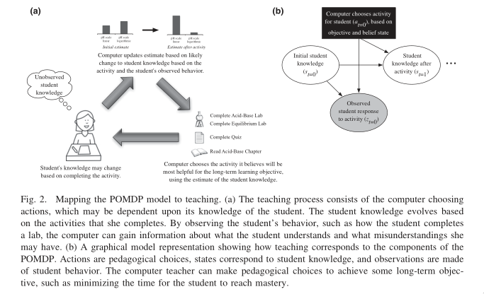
A POMDP is specified as a tuple:

\begin{equation} \langle S, A, Z, p(s'|s, a), p(z|s,a), r(s,a), \gamma \rangle \end{equation}

S

set of states

A

set of actions

Z

set of observations

\(p(s’ | s, a)\)

transition model

\(p(z|s, a)\)

Probability of observing z

\(r(s,a)\)

Reward/cost model

\(\gamma\)

Discount factor

POMDP planning seeks to choose actions that minimize \(\sum_{t=0}^\infty \gamma^t r(s_t, a_t)\).

The learner model specifies the space \(S\) of possible knowledge states, and transition model \(p(s'|s ,a)\) for how knowledge changes.

Simple learner models for concept learning can be specified. For example, in the memoryless model, if an action is consistent with the current concept, then the state stays the same. Else, the learner transitions to a state that is consistent with the action, with probability proportional to the prior probability of the concept:

\begin{equation} p(s_{t+1} = c_i | s_t = c_j , a_t) = \begin{cases} p_0(c_i) & \textrm{ if $c_i$ is consistent with $a_t$} \\\
0 & \textrm{otherwise} \end{cases} \end{equation}

Experiments showed that POMDP planning leads to faster teaching.

Limitations

1. POMDP relies on having models of learning. The models that we currently have do not fully model human learning. Human learners can also learn better if they are aware they are being taught. The models are not accurate enough to know when to decide to terminate teaching. Are we able to learn to teach without explicitly assuming a student model?

2. Beyond time to teach, it is difficult to incorporate other factors such as motivation. The learners may have their own reward function, and a joint optimization of the student and teacher rewards is computationally more difficult.

3. POMDP can be computationally intractable, requiring the use of techniques such as MCTS and forward search, sampling only possible actions taken.

   1. Suppose a task is modelled with a discrete state space. A task with 1000 states will result in a belief state of 1000 dimensions. To overcome this “curse of dimensionality”, point-based POMDP algorithms like HSVI2 and SARSOP use probabilistic sampling.

   2. One can also factor out the fully observable state components to reduce the dimensionality of the belief space into \(S = X \times Y\), where \(X\) is the space of all possible values fully observable variables, and \(Y\) is the space of partially observable variables Du et al., n.d.. Since state variable \(x\) is fully observable, we only need to maintain belief \(b_Y\) for the state variables in \(Y\).

Machine Teaching For Inverse Reinforcement Learning Brown and Niekum, n.d.

Optimal Teaching for IRL gives:

1. Insights into the intrinsic difficulty of teaching certain sequential decision-making tasks
2. Provides a lower bound on the number of samples needed by the active IRL algorithm
3. Optimal teaching can be used to design algorithms that better leverage highly informative demonstrations which do not follow the i.i.d assumptions made by many IRL applications

Machine Teaching Problem for IRL

Given an MDP, \(M\), and the teacher’s reward function, \(R^* = \mathbf{w}^{*^T} \phi (s)\), find the set of demonstrations, \(D\), that minimizes the following optimization problem:

\begin{equation} \textrm{min}_{D} \textrm{TeachingCost}(D) \textrm{ s.t. } \textrm{Loss}(\mathbf{w^*}, \hat{\mathbf{w}}) \le \epsilon, \hat{\mathbf{w}} = IRL(D) \end{equation}

Optimizing this is hard, since there are a large number of candidate sets of demonstrations, and the IRL problem needs to be solved for each candidate set. The paper proposes a greedy set-cover approximation algorithm that requires solving only a single policy-evaluation problem, using the Behavioural Equivalence Class (BEC) of the teacher’s policy.

Teaching Inverse Reinforcement Learners via Features and Demonstrations Haug, Tschiatschek, and Singla, n.d.

It is difficult to specify a reward function that captures all important aspects. In these situations, learning from demonstrations transforms the need of specifying this reward function to the task of providing examples of optimal behaviour.

The paper considers the following setting:

• The true reward function is a linear combination of features known to the teacher
• The learner also assumes the reward function is a linear combination of features, different from the important ones (e.g. observing only a subset)
• The teaching risk is proposed to bound the performance gap of the teacher and learner as a function of the learner’s worldview

Teaching risk is defined as:

\begin{equation} \rho\left(A^{L} ; \mathbf{w}^{*}\right) :=\max _{v \in \operatorname{ker} A^{L},\|v\| \leq 1}\left\langle\mathbf{w}^{*}, v\right\rangle \end{equation}

Where \(A^L\) is the learner’s worldview. Geometrically it is the cosine of the angle between ker \(A^L\) and \(\mathbf{w}^*\).

Limiting the set of teachable features, choosing features that allow for minimizing teaching risk experimentally shows better performance than randomly choosing features.

Learner-aware Teaching: Inverse Reinforcement Learning with Preferences and Constraints Tschiatschek et al., n.d.

This paper considers the setting where the learner has preferences. This captures:

1. behavioural bias
2. mismatched worldviews
3. physical constraints

Learner-aware teaching shows significant performance improvements

Math of the paper is beyond me right now.

Interactive Teaching Algorithms for Inverse Reinforcement Learning Kamalaruban et al., n.d.

Considers the setting where the learner is assisted by a teacher. Two sub-settings are considered:

1. Where the teacher can fully observe the student’s current policy, and understands the student’s dynamics (for theoretical bounds)
2. Where the teacher only has a noisy estimate of the learner’s current policy, and does not understand the student’s dynamics

The environment is modelled as a MDP, where the learner does not have access to the reward furncion R. The teaching objective is to achieve a high-performing policy through learning from teacher demonstrations.

The learner is asssumed to use the MCE-IRL algorithm. Theoretical analysis of the omniscient teacher shows that only \(O(\log \frac{1}{\epsilon})\) demonstrations are required to achieve the teaching objective, an exponential improvement compared to selecting demonstrations at random.

In the black box setting, the strategy considered picks the most informative demonstration. This is evaluated experimentally. The black box teacher is shown to learn faster than the agnostic teacher, in both the linear and non-linear reward setting. In the non-linear reward setting, both learners are unable to learn a good policy, but in the black box teaching setting progress is made much quicker.

Would be interesting to work through the proofs.

Bayesian Teaching

Bayesian teaching aims to induce a target model in the learner by presenting teaching sets of data. This involves two sides of inference:

1. Teacher’s inference: over the space of possible teaching sets
2. Learner’s inference: over the space of possible target models

Bayesian Teaching as Model Explanation

The intuition is that subsets of training data that lead a model to the same (or approximately similar) inference as the model trained on all the data should be useful for understanding the fitted model Sojitra, n.d..

Below is an example of using Bayesian teaching, limited to a teaching set of dimension 2, to understand an MNIST model.

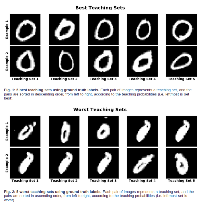
One can inspect the best and worst teaching sets to understand what the model finds to be the best and worst representations for a particular number.

Hence, Bayesian teaching is also useful in telling us which examples are most valuable: better suited to induce the desired target model.

Learning To Interactively Learn and Assist Woodward, Finn, and Hausman, n.d.

Rewards and demonstrations are often defined and collected before training begins, when the human is most uncertain about what information would help the agent.

Key idea: use interactive learning in contrast to rewards or demonstrative learning to enable an agent to learn from another agent who knows the current task.

Interactive learning

Robot Teaching and the Sim2Real gap

Obtaining real-world training data can be expensive, and many RL algorithms are sample-inefficient. Hence, many models are trained in a simulated environment, and the “sim2real” gap causes these models to perform poorly on real-world tasks Weng, n.d..

There are several approaches to closing the sim2real gap:

1. System Identification
   • System identification involves building a mathematical model for a physical system. This requires careful calibration, which can be expensive.
2. Domain Adaptation
   • This refers to a set of transfer learning techniques that update the data distribution in the simulated environment to match that of the real world. Many of these are build on adversarial loss or GAN.
3. Domain Randomization
   • A variety of simulated environments with randomized properties are created, and to allow for training a robust model that works across all these environments.

Both DA and DR are unsupervised. While DA requires a large amount of real data samples to capture the distribution, DR requires little to no real data.

Domain Randomization

Definitions

source domain

The environment we have full access to (the simulator). This is where training happens.

target domain

The environment we want to transfer our model to (the real world)

randomization parameters

A set of parameters in the source domain, which we can sample \(\xi\)

Goal

During policy training, episodes are collected from the source domain with randomization applied. The policy learns to generalize across all the environments. The policy parameter \(\theta\) is trained to maximize the expected reward \(R(\cdot)\) average across a distribution of configurations:

\begin{equation} \theta^{*}=\arg \max _{\theta} \mathbb{E}_{\xi \sim \Xi}\left[\mathbb{E}_{\pi_{\theta}, \tau \sim e_{\xi}}[R(\tau)]\right] \end{equation}

where \(\tau_{\xi}\) is a trajectory collected in the source domain randomized with \(\xi\). Discrepancies between the source and target domains are modelled as variability in the source domain.

In uniform domain randomization, each randomization parameter \(\xi_{i}\) is bounded by an interval \(\xi_{i} \in\left[\xi_{i}^{\mathrm{low}}, \xi_{i}^{\mathrm{high}}\right], i=1, \ldots, N\), and each parameter is uniformly sampled within the range.

• TODO read https://arxiv.org/abs/1703.06907, https://arxiv.org/abs/1611.04201

TODO Domain Randomization as Optimization (read https://arxiv.org/abs/1903.11774)

One can view learning of randomization parameters as a bilevel optimization.

Assume we have access to the real environment \(e_{\textrm{real}}\) and the randomization configuration is sampled from a distribution parameterized by \(\phi\), \(\xi \sim P_{\phi}(\xi)\), we would like to learn a distribution on which policy \(\pi_\theta\) is trained on can achieve maximal performance in \(e_{\textrm{real}}\):

\begin{equation} \begin{array}{c}{\phi^{*}=\arg \min _{\phi} \mathcal{L}\left(\pi_{\theta^{\prime}(\phi)} ; e_{\text { real }}\right)} \ {\text { where } \theta^{*}(\phi)=\arg \min _{\theta} \mathbb{E}_{\xi \sim P_{\phi}(\xi)}\left[\mathcal{L}\left(\pi_{\theta} ; e_{\xi}\right)\right]}\end{array} \end{equation}

where \(\mathcal{L}(\pi ; e)\) is the loss function of policy \(\pi\) evaluated in the environment \(e\).

Guided Domain Randomization

Vanilla Domain Randomization assumes to access to the real data, and randomization configuration is sampled as broadly and uniformly as possible in sim, hoping that the real environment is covered under this broad distribution.

Idea: guide domain randomization to use configurations that are “more realistic”. This avoids training models in unrealistic environments.

TODO read https://arxiv.org/abs/1805.09501

Invariant Risk Minimization Arjovsky et al., n.d.

Key idea: To learn invariances across environments, find a data representation such that the optimal classifier on top of that representation matches for all environments.

Consider a cow/camel classifier. If we train on labeled images where most pictures of cows are taken on green pastures, and pictures of camels in desserts, the classifier may learn to classify green landscapes as cows, and beige landscapes as camels.

To solve this problem, we need to identify which properties of the training data are spurious correlations (e.g. background), and which are actual phenomenon of interest (animal shape). Spurious correlations are expected not to hold in unseen data.

The goal is to learn correlations invariant across training environments.