Interval Estimation in Bayesian Statistics

Suppose instead of point estimation, we’d like to identify a region that is likely to contain the true value of parameter $θ$ . In Bayesian Inference, this region is called the credible set, or the Bayesian confidence interval.

A $100 (1 - α)$ credible set for $θ$ is subset $C$ of $Θ$ such that:

$P (θ \in C | y) = \int_{C} p (θ | y) d θ \geq 1 - α$

Interpreting credible sets is different in Bayesian statistics, compared to frequentist confidence intervals.

In Bayesian statistics, the unknown parameters $θ$ is regarded as a random variable, and the interval is fixed once data is observed. That is, we can make direct probabilistic statements like:

The probability that $θ$ lies in $C$ given observed data $y$ is $(1 - α)$ .

In frequentist statistics, $Y$ is regarded as random, giving rise to a random interval which has probability $(1 - α)$ of containing the fixed but unknown $θ$ . The corresponding statement is:

If we could recompute $C$ for a large number of datasets collected the same way, then about $100 (1 - α)$ of them will contain the true value of $θ$

Another way to view this is that frequentist and Bayesian notions of coverage describe pre- and post-experimental coverage respectively. Researchers have shown that Bayesian credible sets constructed via some methods will also have almost the correct frequentist coverage.

Quantile/equal-tails intervals

We find two numbers $θ_{α / 2} < θ_{1 - α / 2}$ , such that:

$P (θ < θ_{α / 2} | y) = α / 2 and P (θ > θ_{1 - α / 2} | y) = α / 2$

The $100 (1 - α)$ quantile-based CI is $[θ_{α / 2}, θ_{1 - α / 2}]$ .

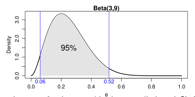
Figure 1: Quantile-based 95% CI for Beta(3,9)

Highest Posterior Density (HPD) region

The HPD credible set is defined as the set:

$C = {θ \in Θ : p (θ | y) \geq k (α)}$

where $k (α)$ is the largest constant satisfying:

$P (θ \in C | y) \geq 1 - α$

All points in a HPD region have higher posterior density than points outside the region.

To visualize this, imagine drawing a horizontal line across the graph at the mode of the posterior distribution, and the pushing it down until the corresponding values on the $θ$ axis contains the appropriate probability.

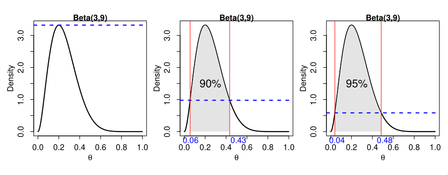
Figure 2: 90% and 95% HPD regions on a Beta(3,9) distribution

Computing HPD requires numerical methods. HPD might not be an interval if the distribution is multimodal. Some packages like coda assumes that the distribution is not severely multimodal.

Generally, the quantile-based CI will be equal to the HPD region if the posterior is symmetric and uni-modal, but wider otherwise. For unimodal posterior densities, the HPD interval has the shortest length for the same level of coverage.