Expectation Maximization and Mixture Models
Introduction
If we define a joint distribution over observed and latent variables, the corresponding distribution of the observed variables alone is obtained by marginalization. This allows relatively complex marginal distributions over observed variables to be expressed in terms of more tractable joint distributions over the expanded space of observed and latent variables.
Mixture distributions, such as the Gaussian mixture, can be interpreted in terms of discrete latent variables. These mixture models are also useful in clustering data. We first discuss the problem of finding clusters using a non-probabilistic technique called K-means clustering. Then we introduce the latent variable view of mixture distributions where the discrete latent variables can be interpreted as defining assignments of data points to specific components of the mixture.
The EM algorithm is the general approach to finding maximum likelihood estimators in latent variable models. We will see that K-means clustering is the non-probabilistic version of the EM algorithm.
K-means Clustering
We formulate the K-means clustering problem as follows:
Suppose we have a datset \(\{\mathbf{x_1}, \dots, \mathbf{x}_N\}\) consisting of \(N\) observations of a random D-dimensional Euclidean variable \(\mathbf{x}\). Our goal is to partition the data set into a fixed number of clusters \(K\). We formalize this by introducing \(\mathbf{\mu}_k\), that represents the center of the clusters. Our goal is then to minimize the objective function:
\begin{equation} J = \sum_{n=1}^{N} \sum_{k=1}^{N} r_{nk} \lvert \mathbf{x}_n - \mathbf{\mu}_k^2 \rvert \end{equation}
The K-means algorithm works as follows:
- Choose some initial values of $μ$_k.
- Minimize \(J\) wrt \(r_{nk}\), keeping \(\mu_k\) fixed.
- Minimize \(J\) wrt \(\mu_k\), keeping \(r_{nk}\) fixed.
- Repeat steps 2 and 3 until convergence.
We shall see that updating \(r_{nk}\) and \(\mu_k\) respectively correspond to the E-step and M-step of the EM algorithm.
Consider first the determination of \(r_{nk}\). Because \(J\) is a ilnear function of \(r_{nk}\), this optimization can be performed easily to give a closed-form solution:
\begin{equation}
r_{nk} = \begin{cases}
1 & \text{if } k = \textrm{argmin}_j \lvert \mathbf{x}_n -
\mathbf{\mu}_j \rvert ^2 \\\
0 & \text{otherwise.}
\end{cases}
\end{equation}
Now, consider the optimization of \(\mu_k\) with \(r_{nk}\) held fixed. The objective function \(J\) is quadratic of \(\mu_k\), and can be minimized by setting the derivative wrt to \(\mu_k\) to 0. We solve it to be:
\begin{equation} \mathbf{\mu}_k = \frac{\sum_{n} r_{nk}\mathbf{x}_n}{\sum_{n} r_{nk}} \end{equation}
This result can be interpreted as setting \(\mu_k\) equal to the mean of all the datapoints \(\mathbf{x}_n\) assigned to cluster \(k\).
Because each step reduces the objective function \(J\), the algorithm is guaranteed to converge to some minimum. This minimum may be a local minimum, instead of a global one.
One way of choosing the cluster centers \(\mu_k\) is to choose a random subset of \(K\) data points as the centers. K-means is often used to initialize parameters in a Gaussian mixture model before applying the EM algorithm.
The K-means algorithm described can be generalized to datasets by using a dissimilarity measure \(\mathcal{V}(x, x’)\) (instead of Euclidean distance), and minimizing the distortion measure:
\begin{equation} \tilde{J} = \sum_{n=1}^{N} \sum_{k=1}^{K} r_{nk}\mathcal{V}(\mathbf{x}_n, \mathbf{x}_k) \end{equation}
which gives the K-medoids algorithm.
The computational cost of the E-step is O(KN), while the M-step involves \(O(N_k^2)\) evaluations of \(\mathcal{V}(\dot, \dot)\).
One feature of the K-means algorithm is that it assigns each datapoint \(\mathbf{x}_i\) to uniquely one of the clusters. There may be datapoints that lie roughly halfway between two cluster centers. By adopting a probabilistic approach, we can obtain ‘soft’ assignments that reflect the level of uncertainty over the most appropriate assignment.
The Gaussian Mixture Model
The Gaussian mixture model allows modelling more complex distributions. We can formulate the Gaussian mixture model in terms of discrete latent variables. the Gaussian mixture distribution can be written as a linear superposition of Gaussians of the form:
\begin{equation} p(\mathbf{x}) = \sum_{k=1}^{K} \pi_k \mathcal{N}(\mathbf{x} | \mathbf{\mu}_k, \mathbf{\Sigma}_k) \end{equation}
We can introduce a K-dimensional binary random variable \(\mathbf{z}\) a 1-of-K representation such that all elements but one of them are 0s, and \(p(z_k = 1) = \pi_k\). We can then define the joint distribution \(p(\mathbf{x}, \mathbf{z})\) corresponding to the following graphical model.
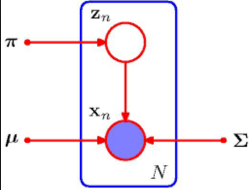
Figure 1: Mixture of Gaussians
The parameters \(\pi_k\) must satisfy:
\begin{equation} 0 \le \pi_k \le 1, \sum_{k=1}^{K}\pi_k = 1 \end{equation}
we can then represent \(p(\mathbf{z})\) as:
\begin{equation} p(\mathbf{z}) = \prod_{k=1}^{K}\pi_k^{z_k} \end{equation}
The conditional distribution can also be written as:
\begin{equation} p(\mathbf{x} | \mathbf{z}) = \prod_{k=1}^{K} \mathcal{N}(\mathbf{x} | \mathbf{\mu}_k, \mathbf{\Sigma}_k)^{z_k} \end{equation}
Since the joint distribution is given by \(p(\mathbf{z})p(\mathbf{x}|\mathbf{z})\), the marginal distribution of \(\mathbf{x}\) is given by summing the joint distribution over all possible states of \(\mathbf{z}\):
\begin{equation} p(\mathbf{x}) = \sum_{z} p(\mathbf{z}) p(\mathbf{x} | \mathbf{z}) = \sum_{k=1}^{K} pi-k \mathcal{N}(\mathbf{x} | \mathbf{\mu}_k, \mathbf{\Sigma}_k) \end{equation}
We define another quantity \(\gamma(z_k) = p(z_k = 1 | \mathbf{x})\), whose quantity can be found via Bayes theorem:
\begin{equation} \gamma(z_k) = \frac{\pi_k \mathcal{N}(\mathbf{x} | \mathbf{\mu}_k, \mathbf{\Sigma}_k)}{\sum_{j=1}^{K} \pi_j \mathcal{N}(\mathbf{x} | \mathbf{\mu}_j, \mathbf{\Sigma}_j)} \end{equation}
We shall view \(\pi_k\) as the prior probability that \(z_k = 1\), and \(\gamma(z_k)\) is the responsibility that component \(k\) takes for explaining the observation \(\mathbf{x}\).
Suppose we have a dataset of observations \(\{\mathbf{x}_1, \dots, \mathbf{x}_k\}\), and wish to model this data using a mixture of Gaussians. We can find the maximum likelihood estimates of the mixture model parameters. Before proceeding, it is worth noting that the maximum likelihood approach has severe problems. In particular, the maximimizing the log likelihood function is not a well-posed problem, and there are singularities that can cause the log-likelihood to become infinity in the limit where the variance is zero. This occurs when a Gaussian component collapses onto a single data point. This can be interpreted as overfitting. We can hope to avoid these singularities by using suitable heuristics, using the MAP or Bayesian approach.
EM for Gaussian Mixture Model
We can find maximum likelihood solutions for models with latent variables using the EM algorithm. We demonstrate this for the case of the Gaussian mixture model.
First, we find the derivatives of \(\ln p(\mathbf{X} | \mathbf{\pi}, \mathbf{\mu}, \mathbf{\Sigma})\) wrt to \(\mu_k\) to 0:
\begin{equation} 0 = \sum_{n=1}^{N} \underbrace{\frac{\pi_k \mathcal{N}(\mathbf{x}_n | \mathbf{\mu}_k, \mathbf{\Sigma}_k)}{\sum_{j} \pi_j \mathcal{N} (\mathbf{x}_n| \mathbf{\mu}_j \mathbf{\Sigma}_j)}}_{\gamma (z_{nk})} \mathbf{\Sigma}^{-1}_k \left( \mathbf{x}_n - \mathbf{\mu}_k \right) \end{equation}
Multiplying by \(\mathbf{\Sigma}_k^{-1}\) (which we assume to be non-singular), we get:
\begin{equation} \mathbf{\mu}_k = \frac{1}{N_k} \sum_{n=1}^{N} \gamma(z_{nk})\mathbf{x}_n, \text{ where } N_k =\sum_{n=1}^{N}\gamma(z_{nk}) \end{equation}
We can interpret \(N_k\) as the effective number of points assigned to cluster \(k\).
If we set the derivative of \(\ln p(\mathbf{X} | \mathbf{\pi}, \mathbf{\mu}, \mathbf{\Sigma})\) wrt to \(\Sigma_k\) to 0, and work it out, we also get that:
\begin{equation} \pi_k = \frac{N_k}{N} \end{equation}
These results are not closed form solutions of the parameters of the mixture model, since they depend on \(\gamma(z_{nk})\). However, the iterative procedure in the EM algorithm, allows us to choose some initial values and perform E and M-steps to converge to a solution.
In the expectation step (E-step), we use the current values for the parameters to evaluate the posterior probabilities, or responsibilities. We then use these probabilities in the maximization step (M-step), to re-estimate the means, covariances and mixing coefficients.
General EM
The goal of the EM algorithm is to find maximum likelihood solutions for models having latent variables. We denote the set of all observed data by \(\mathbf{X}\), in which the nth row represents \(\mathbf{x}_n^T\), and similarly we denote the set of all latent variables by \(Z\), with a corresponding row $\mathbf{z}_n^T4. The set of all model parameters is denoted by \(\mathbf{\theta}\). The log-likelihood function is given by:
\begin{equation} \ln p(\mathbf{X} | \mathbf{\theta}) = \ln \left\{ \sum_{\mathbf{z}} p(\mathbf{X}, \mathbf{Z} | \mathbf{\theta} ) \right\} \end{equation}
A key observation is that the summation occurs within the logarithm. Even if the joint distribution belongs to the exponential family, the marginal \(p(\mathbf{X} | \mathbf{\theta})\) generally does not because of this summation. The presence of the sum prevents the logarithm from acting directly on the joint distribution, resulting in complicated expressions for the maximum likelihood solution.
Since we are in general not given the complete dataset \(\{\mathbf{X}, \mathbf{Z}\}\), but only the incomplete data \(\mathbf{X}\), our state of knowledge of the values of the latent variables is given only by a posterior distribution \(p(\mathbf{Z} | \mathbf{X}, \mathbf{\theta})\). Instead, we consider the expected value under the posterior distribution of the latent variable, which corresponds to the E-step of the EM algorithm. In the subsequent M-step, we maximize this expectation.
In the E-step, we use the current parameters \(\theta^{\text{old}}\) to find the posterior distribution of the latent variables given by \(p(\mathbf{Z} | \mathbf{X}, \mathbf{\theta}^{\text{old}})\). We use the posterior distribution to fin the expectation of the complete-data log likelihood evaluated for some general parameter \(\theta\). This expectation, denoted \(Q(\mathbf{\theta}, \mathbf{\theta}^{\text{old}} )\), is given by:
\begin{equation} Q(\mathbf{\theta}, \mathbf{\theta}^{\text{old}}) = \sum_{\mathbf{Z}} p(\mathbf{Z} | \mathbf{X}, \mathbf{\theta}^{\text{old}})\ln p(\mathbf{X} , \mathbf{Z} | \mathbf{\theta}) \end{equation}
In the M-step, we revise the parameter estimate \(\mathbf{\theta}^{\text{new}}\) by maximizing the Q function:
\begin{equation} \mathbf{\theta}^{\text{new}} = \textrm{argmax}_{\theta} Q(\mathbf{\theta}, \mathbf{\theta}^{\text{old}}) \end{equation}
In the definition of \(Q\), the logarithm acts directly on the joint distribution, making the M-step tractable.
In general, we suppose that the direct optimization of \(p(\mathbf{X} | \mathbf{\theta})\) is difficult, and the optimization of \(p(\mathbf{X}, \mathbf{Z} | \mathbf{\theta})\) is significantly easier.
We introduce a distribution \(q(\mathbf{Z})\) over the latent variables, and we observe that for any choice of \(q(\mathbf{Z})\), the following decomposition holds:
\begin{equation} \ln p(\mathbf{X} | \mathbf{\theta}) = \mathcal{L}(q, \mathbf{\theta}) + KL(q || p) \end{equation}
where
\begin{equation} \mathcal{L} (q, \mathbf{\theta}) = \sum_{\mathbf{Z}} q(\mathbf{Z}) \ln \left\{ \frac{p(\mathbf{X}, \mathbf{Z} | \mathbf{\theta})}{q(\mathbf{Z})} \right\} \end{equation}
and
\begin{equation} KL(q||p) = - \sum_{\mathbf{Z}} q(\mathbf{Z}) \ln \left\{ \frac{p(\mathbf{Z} | \mathbf{X}, \mathbf{\theta})}{q(\mathbf{Z})} \right\} \end{equation}
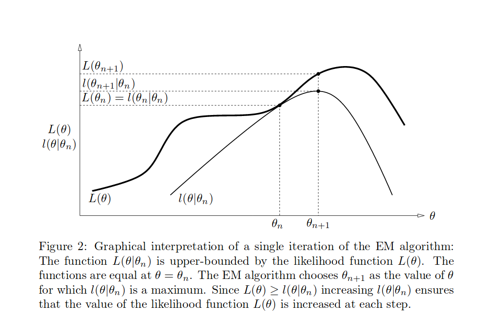
The EM algorithm involves alternatingly computing a lower bound on the log likelihood for the current parameter values, and then maximizing this bound to obtain the new parameter values.
For complex models, the E-step and M-step can still be intractable. The Generalized EM (GEM) algorithm addresses the problem on the intractable M-step. Instead of maximizing \(L(q, \mathbf{\theta})\) wrt \(\mathbf{\theta}\), it seeks to change the parameters such that the value is increased. Similarly, one can address the intractable E-step by seeking to partially optimize \(L(q, \mathbf{\theta})\) wrt \(q(\mathbf{Z})\).
Bishop, n.d.; Borman, n.d.